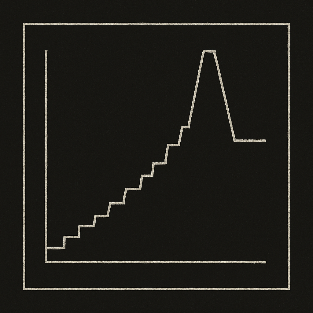
THE MACHINERY OF THRESHOLDS
A Complete Guide to the Gate Between States
How Phase Boundaries Actually Work
What follows is not advice.
It is not a framework for “tipping the balance.” Not a playbook for crossing finish lines. Not a self-help metaphor about breaking through barriers.
It is mechanism.
The actual machinery of the gate. The physics of why systems sit still for a long time and then change all at once. The mathematics of why gradual pressure produces sudden rupture. The architecture that separates the world into before and after.
Thresholds are everywhere. In chemistry, neurons, epidemics, networks, lasers, ecosystems, societies. Every one of them obeys the same structural logic.
Most people think of thresholds as points on a scale. A line you cross if you push hard enough.
This is not what they are.
A threshold is a phase boundary. A gate between two qualitatively different states of being. And the machinery of that gate has rules that hold from atoms to civilizations.
This document is those rules.
Nothing more.
What you do with them is your business.
PART ONE: THE GATE
What a Threshold Actually Is
A threshold is not a number on a dial.
It is a structural discontinuity. A point where the relationship between input and output changes qualitatively. Where more of the same becomes something different entirely.
Below the threshold, increasing the input produces proportional response. Linear. Predictable. Boring.
At the threshold, the system reorganizes. New behavior emerges that did not exist at any level below. Not more of the old thing. A different thing.
Water at 99 degrees Celsius is hot liquid. Water at 100 degrees is steam. The single degree is not what matters. What matters is that the system crossed a phase boundary where the rules changed.
    THE STRUCTURE OF A THRESHOLD

    Response
         │
         │                                    ████████
         │                                ████
    HIGH │                              ██
         │                             █
         │                            █
         │                           █  ← THRESHOLD
         │                          █     (phase boundary)
    MED  │                        ██
         │                      ██
         │                   ███
         │               ████
    LOW  │  █████████████
         │
         └──────────────────────────────────────────────►
                                                   Input
           GRADUAL                │            NEW STATE
           ACCUMULATION          │            (qualitatively
                                 │             different)
The sigmoid. The S-curve. The step function.
Every threshold in nature draws this shape.
Gradual, gradual, gradual. Then sudden. Then stable again.
The sudden part is not an accident. It is the signature of a phase boundary being crossed. It appears in neurons and nations, in chemical reactions and social revolutions, in crystal formation and information channels.
Same shape. Same logic. Different substrate.
The Heaviside Function
The simplest mathematical threshold is the Heaviside step function.
Below zero: output is zero. At zero: the step. Above zero: output is one.
Nothing, nothing, nothing. Everything.
    THE HEAVISIDE STEP FUNCTION

    Output
         │
       1 │                    ┌──────────────────
         │                    │
         │                    │
         │                    │
         │                    │
       0 │────────────────────┘
         │
         └────────────────────┬──────────────────►
                              0              Input

         ALL-OR-NOTHING: the purest threshold
Real systems smooth this into a sigmoid. The transition zone has finite width. But the logic is the same. Below some critical value, the system is in one state. Above it, another. The transition between them is steep relative to the scale of the input.
This is the mathematical atom of discontinuous change.
Every threshold in this document is a variation on this shape. What varies is the substrate, the mechanism that creates the steepness, and the consequences of crossing.
PART TWO: THE ENERGY BARRIER
Activation Energy
The oldest and clearest threshold in science is the activation energy barrier.
Svante Arrhenius formalized this in 1889. For a chemical reaction to proceed, the reactant molecules must have enough kinetic energy to reach a transition state. Below that energy, nothing happens. The molecules collide and bounce apart. Above it, the reaction proceeds. Bonds break. New bonds form. Products appear.
The activation energy is the height of the hill between the reactant valley and the product valley.
    THE ENERGY LANDSCAPE

    Free
    Energy
         │
         │           ┌───┐
         │          ╱     ╲
         │         ╱       ╲          Ea = Activation
         │        ╱         ╲              Energy
         │       ╱    Ea     ╲
         │      ╱     ↕       ╲
    ─────┼─────╱               ╲
         │    ╱                 ╲
         │   REACTANTS           ╲
         │                        ╲──────────
         │                        PRODUCTS
         │
         └──────────────────────────────────────────►
                   Reaction Coordinate
The Arrhenius equation quantifies this:
k = A · e^(-Ea/RT)
Where k is the reaction rate, A is the attempt frequency, Ea is the activation energy, R is the gas constant, and T is the temperature.
The exponential term is what matters. It means the rate increases not linearly but exponentially with temperature. A small increase in temperature near the threshold produces an enormous increase in reaction rate. Below a certain temperature, the rate is effectively zero. Above it, the reaction proceeds vigorously.
This is why a match head sits stable for years, then ignites in a fraction of a second. The activation energy barrier held the system in metastability. A small local input of energy (friction heat) pushed enough molecules over the barrier. And because combustion releases energy, those molecules push their neighbors over too.
Chain reaction. Cascade. The threshold is not just crossed. It is destroyed by its own crossing.
The Boltzmann Distribution
Why the exponential? Because molecular energies follow the Boltzmann distribution.
At any temperature, most molecules have moderate energy. A few have very high energy. The fraction with energy above any given threshold drops exponentially with the height of that threshold.
    BOLTZMANN DISTRIBUTION AT TWO TEMPERATURES

    Fraction
    of
    Molecules
         │
         │█
         │██
         │████
         │██████  ← LOW TEMPERATURE
         │█████████
         │████████████
         │██████████████████
         │                          ██
         │                        ██████  ← HIGH TEMPERATURE
         │                     █████████████
         │                  █████████████████████
         │               ████████████████████████████
         │
         └────────────────┬──────────────────────────►
                          Ea            Energy
                          │
                    ACTIVATION
                    ENERGY
                    THRESHOLD
At low temperature, almost no molecules have enough energy. The reaction rate is negligible.
At high temperature, a significant fraction exceeds the barrier. The reaction proceeds.
The threshold itself does not move. What changes is how many entities have enough energy to cross it.
This is a universal principle. Thresholds are not always about whether something can happen. They are about whether enough things happen simultaneously for the collective effect to matter.
PART THREE: THE BIFURCATION
When Stable Becomes Unstable
In dynamical systems theory, the most important threshold is the bifurcation point.
A bifurcation occurs when a small smooth change in a parameter causes a qualitative change in the system’s behavior. A stable state that existed for all previous parameter values suddenly ceases to exist. Or a new stable state appears from nowhere.
The most common type is the saddle-node bifurcation.
Two equilibria exist: one stable (the node), one unstable (the saddle). As a parameter changes, they move toward each other. At the bifurcation point, they collide and annihilate. The stable state vanishes.
    SADDLE-NODE BIFURCATION

    System
    State
         │
         │   ●━━━━━━━━━━━━━━━━●
         │   stable            │    (stable and unstable
         │                     │     equilibria merge)
         │   ○╌╌╌╌╌╌╌╌╌╌╌╌╌╌╌○
         │   unstable          │
         │                     │
         │                     ▼
         │                     ╳  ← BIFURCATION POINT
         │                     │
         │                     │    (both equilibria
         │                     │     annihilate)
         │                     │
         │                     ▼
         │
         │              NO EQUILIBRIUM
         │              System collapses
         │              to distant state
         │
         └──────────────────────────────────────────►
                          Parameter value
This is the mathematics of the tipping point.
Before the bifurcation, the system has a place to rest. After, it does not. The state it occupied no longer exists. It must fall to wherever the next attractor lies, which may be very far from where it was.
This is not gradual change. It is structural collapse. The floor disappears.
Ecosystems, climate systems, financial markets, and mechanical structures all exhibit this pattern. The load on a beam increases slowly. The beam holds. Holds. Holds. Then buckles. The buckling is not the last increment of load. It is the annihilation of the equilibrium.
The Point of No Return
A feature of saddle-node bifurcation is hysteresis.
Once the system has fallen past the threshold to a new state, reversing the parameter to its original value does not bring the system back. The forward threshold and the backward threshold are at different parameter values.
    HYSTERESIS: THE ASYMMETRY OF CROSSING

    System
    State
         │
         │   STATE A ━━━━━━━━━━━━━━━━┓
         │                            ┃
         │                            ┃ FORWARD
         │                            ┃ THRESHOLD
         │                            ┃
         │                            ▼
         │        ┏━━━━━━━━━━━━━━━━━━━━━━━━ STATE B
         │        ┃
         │        ┃ BACKWARD
         │        ┃ THRESHOLD
         │        ┃
         │        ┃
         │
         └────────┼───────────────────┼─────────────►
                  │                   │     Parameter
              RECOVERY            COLLAPSE
              POINT               POINT

         The gap between them is the hysteresis zone.
         Crossing forward is easy. Getting back is hard.
This is why ecosystem collapses are so difficult to reverse. Why recessions persist long after the trigger is removed. Why a broken trust does not repair when the offending behavior stops.
The system crossed a threshold that reshaped the landscape itself. The return path is not the same as the forward path. It may require far more extreme conditions, or the original state may be permanently inaccessible.
Thresholds are not symmetric. Crossing them changes the terrain.
PART FOUR: THE PERCOLATION POINT
The Giant Component
In a random network, nodes connect to other nodes with some probability p.
When p is low, the network consists of small, isolated clusters. Local connections. No global structure.
As p increases, clusters grow. They merge. But nothing qualitative changes.
Then, at a critical probability p_c, something sudden happens. The small clusters link together into a single giant component that spans the entire network. Not gradually. Abruptly.
    PERCOLATION THRESHOLD

    Size of
    Largest
    Cluster
         │
         │                              ████████████
         │                           ███
         │                         ██
         │                        █  ← PERCOLATION
         │                       █     THRESHOLD (p_c)
         │                      █
         │                    ██
         │                 ███
    SMALL│ ████████████████
         │
         └──────────────────────────────────────────►
           0                p_c               1.0
                   Connection Probability

    Below p_c: isolated clusters
    Above p_c: a giant connected component emerges
This is a geometric phase transition. Below the threshold, information (or disease, or fire, or electrical current) can only travel short distances. Above it, it can traverse the entire system.
The percolation threshold for a two-dimensional square lattice is approximately 0.5927 for site percolation. For a triangular lattice, exactly 0.5. The precise value depends on the geometry of the network, but the existence of a sharp threshold is universal.
At the threshold itself, the system is fractal. The largest cluster has a self-similar structure with holes at every scale. Neither connected nor disconnected. Poised at the boundary between local and global.
This is not a metaphor for how connectivity works.
It is how connectivity works.
What Percolation Teaches
The percolation threshold reveals something fundamental about thresholds in general.
The transition is not caused by any single connection. No individual link “tips” the system. The threshold is a collective phenomenon. It emerges from the statistical accumulation of local events into a global structural change.
    LOCAL VS GLOBAL

    ┌──────────────────────────┐      ┌──────────────────────────┐
    │                          │      │                          │
    │  BELOW THRESHOLD         │      │  ABOVE THRESHOLD         │
    │                          │      │                          │
    │    ●─●  ●─●              │      │    ●─●─●─●─●─●           │
    │         ●                │      │    │   │     │           │
    │    ●─●     ●─●           │      │    ●─●─●   ●─●           │
    │                          │      │        │ │               │
    │    ●    ●─●─●            │      │    ●─●─●─●─●             │
    │                          │      │                          │
    │  Local clusters only     │      │  Global connectivity     │
    │  No spanning path        │      │  Spanning path exists    │
    │                          │      │                          │
    └──────────────────────────┘      └──────────────────────────┘
This principle extends far beyond random graphs. Forest fires spread through percolation of flammable trees. Epidemics spread through percolation of susceptible contacts. Ideas spread through percolation of receptive minds. Current flows through percolation of conductive particles.
The question is never “is this connection enough?” The question is “has the network reached the density where a spanning path exists?”
PART FIVE: THE ALL-OR-NOTHING GATE
The Action Potential
The neuron is a threshold machine.
The membrane rests at approximately -70 millivolts. Inputs arrive. Small depolarizations. They accumulate, summing at the axon hillock. If the cumulative depolarization reaches approximately -55 millivolts, voltage-gated sodium channels open.
Sodium floods in. The membrane depolarizes further. This opens more sodium channels. More sodium. More depolarization. More channels.
Positive feedback. Explosion. The membrane potential shoots to +40 millivolts in less than a millisecond.
This is the action potential. And it is all-or-nothing.
    THE NEURAL THRESHOLD

    Membrane
    Potential
    (mV)
         │
     +40 │                 ┌──┐
         │                ╱    ╲
         │               ╱      ╲
         │              ╱        ╲
      0  │─────────────╱──────────╲──────────────
         │            ╱            ╲
         │           ╱              ╲───────
    -55  │──────────╱─── THRESHOLD ─────────────
         │         ╱
    -70  │────────╱── RESTING POTENTIAL
         │       ╱
         │      ╱
         │   subthreshold
         │   inputs
         │
         └──────────────────────────────────────►
                                          Time

    Below -55mV: nothing happens, membrane returns to rest
    At -55mV: positive feedback triggers full depolarization
Below threshold, the input dissipates. The membrane returns to rest. No signal is sent.
At threshold, the system fires with full amplitude. A subthreshold input of -56 mV and a suprathreshold input of -54 mV differ by 2 millivolts. But their outputs differ categorically. Zero versus full signal. Silence versus transmission.
The mechanism is positive feedback through voltage-gated channels. The threshold is the point where positive feedback overwhelms negative feedback. Where the inward sodium current exceeds the outward potassium current. Where gain exceeds loss.
This is the same structure as the laser.
The Laser Threshold
A laser medium contains atoms in excited states. They emit photons. But most photons escape the cavity or are absorbed. The medium also absorbs light, stealing photons.
Pump more energy in. More atoms reach excited states. The ratio of excited to ground-state atoms increases. When it crosses a critical value, a population inversion, gain exceeds loss.
At this point, every photon that triggers stimulated emission creates another photon that triggers more stimulated emission. Positive feedback. Cascade. The light intensity grows exponentially until it saturates.
Below threshold: dim, incoherent fluorescence. Above threshold: coherent, monochromatic laser light.
    THE LASER THRESHOLD

    Light
    Output
         │
         │                              ████████████
         │                            ██
         │                          ██
         │                        ██
         │                      ██
         │                    ██
         │                   █  ← LASER THRESHOLD
         │                  █     (gain = loss)
         │               ███
    GLOW │ ██████████████
         │ (fluorescence)
         │
         └──────────────────────────────────────────►
                              Pump Power

    Below threshold: spontaneous emission (random, dim)
    Above threshold: stimulated emission (coherent, intense)
The pattern repeats.
The neuron fires when inward current exceeds outward current. The laser fires when gain exceeds loss. The chemical reaction proceeds when molecular energy exceeds the activation barrier. The network percolates when connection density exceeds the critical fraction.
Same structure. Gain exceeds loss. Positive feedback overpowers negative feedback. The system transitions.
PART SIX: THE INFORMATION BOUNDARY
Shannon’s Limit
In 1948, Claude Shannon proved something that should have been impossible to prove.
For any communication channel with a given noise level, there exists a maximum rate at which information can be transmitted with arbitrarily low error probability. This is the channel capacity.
Below capacity, error-free communication is possible. Codes exist that can correct the noise.
Above capacity, reliable communication is impossible. No code can save you. Errors are inevitable and uncorrectable.
    THE SHANNON THRESHOLD

    Error
    Probability
         │
       1 │████████████████
         │                ████
         │                    ████
         │                        ████
         │                            ████
         │                                ████
         │                                    ████
         │                                        ████
       0 │────────────────────────────────────────────████████
         │
         └────────────────────────┬──────────────────────────►
                                  C          Transmission Rate

         Below C: error can be made           Above C: error
         arbitrarily small                    is unavoidable
This is not an engineering limitation. It is a mathematical law. No future technology, no cleverer encoding, no amount of processing power can transmit reliably above the channel capacity. The threshold is absolute.
Shannon proved the existence of good codes but did not construct them. It took sixty years for turbo codes and LDPC codes to approach the limit in practice. The threshold was real all along. The engineering just had to catch up to the mathematics.
The Shannon limit is a threshold with no ambiguity. On one side, perfection is achievable. On the other, it is provably impossible. The transition is sharp. This is the cleanest threshold in all of science.
What Information Thresholds Teach
The Shannon limit reveals that thresholds can be absolute boundaries, not just difficult-to-cross barriers. Some thresholds separate the possible from the impossible.
This distinction matters.
An activation energy barrier can be overcome by adding more energy. A percolation threshold can be crossed by adding more connections. These are barriers of degree.
The Shannon limit is a barrier of kind. No amount of effort changes which side you are on. You either operate below capacity or you do not.
Nature contains both types. Knowing which type you face changes everything about the appropriate response.
PART SEVEN: THE CONTAGION THRESHOLD
R0 and the Epidemic Threshold
In epidemiology, the basic reproduction number R0 is the average number of secondary infections produced by a single infected individual in a fully susceptible population.
R0 = 1 is the epidemic threshold.
Below 1: each infected person infects fewer than one other on average. The disease dies out. Exponential decay.
Above 1: each infected person infects more than one other. The disease spreads. Exponential growth.
    THE EPIDEMIC THRESHOLD

                     R0 < 1                              R0 > 1

              ●                                    ●
             ╱                                    ╱ ╲
            ●                                    ●   ●
                                                ╱ ╲ ╱ ╲
          (dies out)                            ●  ● ●  ●
                                               ╱╲ ╱╲ ╱╲ ╱╲
                                              ● ●● ●● ●● ●

                                             (exponential spread)


    Infected
    Count
         │
         │                                  ╱╱╱  R0 = 2.5
         │                                ╱╱
         │                              ╱╱
         │                            ╱╱
         │                          ╱╱
         │                        ╱╱        ───── R0 = 1.1
         │                      ╱╱     ─────
         │                    ╱╱──────
         │               ╱╱╱─
         │          ╱╱╱╱──── ╲╲╲╲  R0 = 0.9
         │    ╱╱╱╱╱─               ╲╲╲╲╲╲
         │╱╱╱╱                              ╲╲╲╲  R0 = 0.5
         └──────────────────────────────────────────────────►
                                                        Time
The difference between R0 = 0.99 and R0 = 1.01 is the difference between extinction and pandemic. Two hundredths of a reproduction number. But the qualitative outcome is binary.
This is the threshold at work. Not a smooth transition. A phase boundary between die-out and take-over.
Granovetter’s Threshold Model
In 1978, Mark Granovetter extended threshold logic to collective human behavior.
Each individual in a population has a personal threshold: the fraction of others who must adopt a behavior before that individual will adopt it too. Some people have low thresholds (early adopters, risk-takers). Some have high thresholds (they need to see most others doing it first).
The population-level dynamics depend not on the average threshold but on the distribution.
    GRANOVETTER'S CASCADE

    Number
    of
    People
         │
         │    ██
         │    ██ ██
         │    ██ ██ ██
         │ ██ ██ ██ ██ ██
         │ ██ ██ ██ ██ ██ ██
         │ ██ ██ ██ ██ ██ ██ ██
         │ ██ ██ ██ ██ ██ ██ ██ ██ ██
         │
         └──────────────────────────────────────────►
           0%    20%    40%    60%    80%    100%
                   Individual Threshold

    If this distribution has no gaps: full cascade
    If a gap exists at any point: cascade stalls there
A population where thresholds are uniformly distributed from 0% to 100% will cascade completely. Person with threshold 0 starts. This triggers person with threshold 1%. They trigger 2%. The chain is unbroken.
But if no one has a threshold of, say, 25%, the cascade stalls at 24%. A quarter of the population adopts. The rest never do. Despite being “willing” at higher thresholds, they never see the fraction they need.
The system-level threshold emerges from the distribution of individual thresholds. It is a gap in the chain. A break in the percolation path. Where it breaks determines whether you get riot or peace, adoption or stagnation, revolution or murmur.
Same collective phenomenon. Same structural threshold. Applied to human populations.
PART EIGHT: THE NUCLEATION BARRIER
The Critical Radius
First-order phase transitions do not happen everywhere at once.
They begin as nuclei. Tiny seeds of the new phase forming within the old. A droplet of liquid in supersaturated vapor. A crystal forming in supersaturated solution. A bubble of gas in superheated liquid.
But small nuclei are unstable. The surface energy penalty of maintaining the boundary between old phase and new phase dominates. The nucleus dissolves back into the old phase.
Only nuclei above a critical radius are stable. Below it, surface tension wins. Above it, the volume energy of the new phase wins. The nucleus grows without limit.
    THE NUCLEATION ENERGY BARRIER

    Free
    Energy
    Change
         │
         │         ┌────┐
         │        ╱      ╲
         │       ╱   ΔG*  ╲           ΔG* = Critical
     (+) │      ╱    ↕      ╲              barrier height
         │     ╱              ╲
         │    ╱                ╲
    ─────┼───╱──────────────────╲────────────────
         │  ╱                    ╲
     (-) │ ╱       r*             ╲
         │╱                        ╲
         │     CRITICAL              ╲──────────
         │     RADIUS                 STABLE
         │                            GROWTH
         │
         └──────────────────────────────────────────►
                          Nucleus Radius (r)

    Below r*: nucleus dissolves (surface term dominates)
    Above r*: nucleus grows (volume term dominates)
This creates a threshold with a specific character: the system must fluctuate over a barrier to reach the new state. It is not enough to merely prefer the new state thermodynamically. The system must assemble a nucleus of sufficient size in a single fluctuation.
This is why supercooled water can remain liquid below 0°C. The ice phase is thermodynamically favored, but no nucleus of sufficient size has formed. The system is trapped in a metastable state by the nucleation barrier.
Shake the container. Introduce a seed crystal. Scratch the surface to provide a nucleation site. The barrier is overcome and ice propagates through the entire volume in seconds.
The lesson: a threshold can separate a system from its preferred state indefinitely. The system “wants” to transition. The thermodynamics demand it. But the nucleation barrier stands between wanting and happening. Only a sufficiently large fluctuation, or an external perturbation, opens the gate.
PART NINE: CRITICAL SLOWING DOWN
The System Tells You Before It Tips
In 2009, Marten Scheffer and colleagues published a landmark paper identifying generic early warning signals of approaching thresholds.
The key insight: systems approaching a bifurcation point slow down.
When a system is far from its threshold, perturbations decay quickly. Push it off its equilibrium and it snaps back. The recovery is fast. The basin of attraction is deep and steep.
As the system approaches the threshold, the basin shallows. The equilibrium becomes weaker. Perturbations take longer to decay. The system drifts more before recovering. Its memory of past states increases. Its fluctuations grow larger.
    THE BASIN SHALLOWS NEAR THE THRESHOLD

    FAR FROM THRESHOLD         APPROACHING THRESHOLD

    ╲          ╱               ╲                    ╱
     ╲        ╱                 ╲                  ╱
      ╲      ╱                   ╲                ╱
       ╲    ╱                     ╲              ╱
        ╲  ╱                       ╲            ╱
         ╲╱   ← deep basin          ╲          ╱
          ●                           ╲        ╱
                                       ╲      ╱
        FAST                            ╲    ╱
        RECOVERY                         ╲  ╱
                                          ╲╱  ← shallow basin
                                           ●

                                         SLOW
                                         RECOVERY
Three measurable signals emerge:
Rising autocorrelation. Each state increasingly resembles the previous one. The system loses its ability to “forget” perturbations.
Rising variance. Fluctuations grow larger because the restoring force is weaker.
Rising skewness. The system starts to flicker toward the alternative state, producing asymmetric fluctuations.
    EARLY WARNING SIGNALS

    TIME SERIES FAR FROM THRESHOLD:

    ─────────╱╲─────╱╲───────╱╲──────╱╲───────────
              Small, fast          Small, fast
              fluctuations        fluctuations


    TIME SERIES NEAR THRESHOLD:

                          ╱╲
                    ╱╲   ╱  ╲         ╱╲
              ╱╲  ╱  ╲ ╱    ╲  ╱╲   ╱  ╲ ╱╲
    ──────╱╲─╱──╲╱────╲╱──────╲╱──╲─╱────╲╱──╲────
           Larger, slower, more correlated
           fluctuations
This is the system whispering that its threshold is close.
The lake that takes longer to clear after each algal bloom. The financial market where volatility clusters and autocorrelation rises. The ecosystem where recovery from each disturbance takes longer.
Critical slowing down is not a metaphor. It is a measurable, quantifiable precursor to threshold crossing. A diagnostic of the approaching gate.
PART TEN: THE CONSTRAINTS
The Four Laws of Thresholds
Every threshold system obeys structural constraints. These are not guidelines. They are properties of the mathematics.
    ┌──────────────────────────────────────────────────────────┐
    │                                                          │
    │   CONSTRAINT 1: NONLINEARITY IS REQUIRED                 │
    │                                                          │
    │   Linear systems have no thresholds.                     │
    │   Double the input, double the output.                   │
    │   No phase boundary exists.                              │
    │   Thresholds require a nonlinear relationship            │
    │   between input and output. Always.                      │
    │                                                          │
    └──────────────────────────────────────────────────────────┘

    ┌──────────────────────────────────────────────────────────┐
    │                                                          │
    │   CONSTRAINT 2: POSITIVE FEEDBACK CREATES THE GATE       │
    │                                                          │
    │   Every sharp threshold involves positive feedback.      │
    │   Sodium channels open more channels.                    │
    │   Infections create more infections.                     │
    │   Connections enable more connections.                   │
    │   The threshold is where positive feedback               │
    │   overpowers negative feedback.                          │
    │                                                          │
    └──────────────────────────────────────────────────────────┘

    ┌──────────────────────────────────────────────────────────┐
    │                                                          │
    │   CONSTRAINT 3: HYSTERESIS IS THE NORM                   │
    │                                                          │
    │   Most thresholds are asymmetric.                        │
    │   Crossing forward is not crossing backward.             │
    │   The system that tips does not un-tip                   │
    │   at the same parameter value.                           │
    │   Often it cannot un-tip at all.                         │
    │                                                          │
    └──────────────────────────────────────────────────────────┘

    ┌──────────────────────────────────────────────────────────┐
    │                                                          │
    │   CONSTRAINT 4: THE THRESHOLD IS A PROPERTY              │
    │   OF THE SYSTEM, NOT THE INPUT                           │
    │                                                          │
    │   The critical temperature depends on the substance.     │
    │   The percolation threshold depends on the lattice.      │
    │   The epidemic threshold depends on the network.         │
    │   The bifurcation point depends on the dynamics.         │
    │   The input merely reaches the gate.                     │
    │   The gate is built into the system itself.              │
    │                                                          │
    └──────────────────────────────────────────────────────────┘
The Universality of Threshold Behavior
Near a continuous phase transition, systems exhibit universal behavior. The critical exponents that describe how quantities diverge near the threshold depend only on a few properties: the dimensionality of the system and the symmetry of the order parameter.
A ferromagnet approaching its Curie temperature and a fluid approaching its critical point exhibit the same critical exponents. Despite being completely different physical systems.
This is universality. It means that thresholds are not merely analogies between different systems. They are the same mathematics wearing different physical costumes.
| System | Threshold | Order Parameter | Universality Class |
|---|---|---|---|
| Water | Boiling point | Density difference | Liquid-gas |
| Magnet | Curie temperature | Magnetization | Ising |
| Network | Percolation point | Giant component size | Percolation |
| Epidemic | R0 = 1 | Fraction infected | Directed percolation |
| Neuron | -55 mV | Firing rate | Excitable media |
| Laser | Gain = loss | Light intensity | Laser |
Different substrates. Same mathematics. Same critical behavior near the threshold. Same power-law scaling. Same diverging correlation lengths.
The threshold is not a metaphor that applies across domains.
It is a mathematical structure that is domain-independent.
PART ELEVEN: THE COMPLETE PICTURE
The Unified Framework
Everything connects.
    THE COMPLETE THRESHOLD FRAMEWORK

    ┌──────────────────────────────────────────────────────────┐
    │                                                          │
    │                    THE THRESHOLD                         │
    │                                                          │
    │    A phase boundary where the relationship between       │
    │    input and output changes qualitatively. Where         │
    │    gradual accumulation produces sudden transition.      │
    │                                                          │
    └──────────────────────────────────────────────────────────┘
                              │
              ┌───────────────┼───────────────┐
              │               │               │
              ▼               ▼               ▼
    ┌────────────────┐ ┌────────────────┐ ┌────────────────┐
    │                │ │                │ │                │
    │   BARRIERS     │ │  BIFURCATIONS  │ │   CASCADES     │
    │                │ │                │ │                │
    │  Activation    │ │  Saddle-node   │ │  Percolation   │
    │  energy.       │ │  collapse.     │ │  threshold.    │
    │  Nucleation    │ │  Tipping       │ │  Epidemic      │
    │  radius.       │ │  points.       │ │  threshold.    │
    │  Shannon       │ │  Regime        │ │  Granovetter   │
    │  limit.        │ │  shifts.       │ │  cascades.     │
    │                │ │                │ │                │
    └────────────────┘ └────────────────┘ └────────────────┘
              │               │               │
              └───────────────┼───────────────┘
                              │
                              ▼
    ┌──────────────────────────────────────────────────────────┐
    │                                                          │
    │                   THE GATE OPENS                         │
    │                                                          │
    │    Positive feedback overpowers negative feedback.       │
    │    The old state becomes unstable or inaccessible.       │
    │    The system reorganizes into a qualitatively           │
    │    different configuration.                              │
    │                                                          │
    └──────────────────────────────────────────────────────────┘
An activation energy barrier is a gate you must push through. The system needs enough energy concentrated in the right place at the right time. Chemistry. Nucleation. Ignition.
A bifurcation is a gate that disappears. The system does not push through anything. The floor it was standing on ceases to exist. Ecosystem collapse. Structural buckling. Market crashes.
A cascade threshold is a gate that opens from within. Once enough elements have transitioned, they pull the rest. Epidemics. Network connectivity. Social contagion.
Three flavors of the same structural phenomenon.
The Operating Principles
    THE TWO OPERATING MODES

    ════════════════════════════════════════════════════════════

    MODE A: APPROACHING A THRESHOLD

    What accumulates:
    • Energy concentrates (activation barriers)
    • Parameters drift (bifurcations)
    • Connections form (percolation)
    • Adopters increase (cascades)

    Warning signals:
    • Critical slowing down
    • Rising variance and autocorrelation
    • Flickering between states
    • Longer recovery from perturbations

    ════════════════════════════════════════════════════════════

    MODE B: HOLDING A THRESHOLD

    What prevents crossing:
    • Dissipating energy before it accumulates
    • Maintaining distance from bifurcation point
    • Keeping connections below percolation density
    • Breaking the chain in cascade sequences

    Stabilizing mechanisms:
    • Negative feedback dominance
    • Deep basins of attraction
    • Redundancy and buffering
    • Heterogeneity in threshold distributions

    ════════════════════════════════════════════════════════════
These are not recommendations. They are descriptions of what happens.
Systems approach thresholds through accumulation. They resist thresholds through dissipation. The balance between these two processes determines whether and when the gate opens.
Final Synthesis
A threshold is not a line on a graph.
It is the boundary between two qualitatively different states of organization. The gate where positive feedback overwhelms negative feedback. Where the old equilibrium becomes unstable. Where the spanning path finally connects.
The physics is the same everywhere.
Activation energy in chemistry. Bifurcation points in dynamical systems. Percolation thresholds in networks. R0 = 1 in epidemiology. -55 millivolts in neurons. Gain equals loss in lasers. Channel capacity in information theory. Critical nucleus size in phase transitions.
Different substrates. Same gate.
Below the threshold, the system absorbs input. Dissipates it. Returns to rest. Nothing visible happens, no matter how much force is applied. This is not resistance. It is the system operating in a regime where negative feedback dominates.
At the threshold, positive feedback takes over. The system cannot return to rest. The old state is either destroyed (bifurcation), overwhelmed (cascade), or escaped (barrier crossing). A new state emerges.
Above the threshold, the system is in a different world. Different rules. Different dynamics. Different possibilities. And often, a different threshold for return. Or no return path at all.
The accumulation before the threshold is invisible. The transition is sudden. The new state is stable. This is not a story about tipping points. It is the mathematics of how states change.
Ice becoming water. Networks becoming connected. Populations becoming infected. Neurons becoming active. Lasers becoming coherent.
The same gate. The same physics. The same machinery.
Operating everywhere. Always. Whether anyone is watching or not.
CITATIONS
Phase Transitions and Critical Phenomena
Critical Phenomena and Universality
Kadanoff, L.P. (2009). “More is the Same; Phase Transitions and Mean Field Theories.” Journal of Statistical Physics, 137(5-6):777-797. https://arxiv.org/abs/0906.0653
Stanley, H.E. (1999). “Scaling, universality, and renormalization: Three pillars of modern critical phenomena.” Reviews of Modern Physics, 71(2):S358-S366. https://journals.aps.org/rmp/abstract/10.1103/RevModPhys.71.S358
Phase Transitions Overview
“Phase transition.” Wikipedia. https://en.wikipedia.org/wiki/Phase_transition
“Critical phenomena.” Wikipedia. https://en.wikipedia.org/wiki/Critical_phenomena
Activation Energy and Chemical Kinetics
Arrhenius Equation
Arrhenius, S. (1889). “Über die Reaktionsgeschwindigkeit bei der Inversion von Rohrzucker durch Säuren.” Zeitschrift für physikalische Chemie, 4:226-248.
“Arrhenius Equation.” Chemistry LibreTexts. https://chem.libretexts.org/Bookshelves/Physical_and_Theoretical_Chemistry_Textbook_Maps/Supplemental_Modules_(Physical_and_Theoretical_Chemistry)/Kinetics/06:_Modeling_Reaction_Kinetics/6.02:_Temperature_Dependence_of_Reaction_Rates/6.2.03:_The_Arrhenius_Law/6.2.3.01:_Arrhenius_Equation
Bifurcation Theory and Tipping Points
Saddle-Node Bifurcation
Strogatz, S.H. (2015). Nonlinear Dynamics and Chaos. 2nd Edition. Westview Press.
Ritchie, P. & Sieber, J. (2016). “Time-dependent saddle-node bifurcation: Breaking time and the point of no return in a non-autonomous model of critical transitions.” Proceedings of the Royal Society A. https://pmc.ncbi.nlm.nih.gov/articles/PMC6836434/
Bifurcation Theory
“Bifurcation theory.” Wikipedia. https://en.wikipedia.org/wiki/Bifurcation_theory
Percolation Theory
Percolation Threshold
Broadbent, S.R. & Hammersley, J.M. (1957). “Percolation processes: I. Crystals and mazes.” Mathematical Proceedings of the Cambridge Philosophical Society, 53(3):629-641.
Stauffer, D. & Aharony, A. (1994). Introduction to Percolation Theory. 2nd Edition. Taylor & Francis.
“Percolation threshold.” Wikipedia. https://en.wikipedia.org/wiki/Percolation_threshold
Neuroscience
Action Potential and Threshold
Hodgkin, A.L. & Huxley, A.F. (1952). “A quantitative description of membrane current and its application to conduction and excitation in nerve.” The Journal of Physiology, 117(4):500-544.
“Physiology, Action Potential.” StatPearls, NCBI Bookshelf. https://www.ncbi.nlm.nih.gov/books/NBK538143/
Laser Physics
Laser Threshold
Siegman, A.E. (1986). Lasers. University Science Books.
“Lasing threshold.” Wikipedia. https://en.wikipedia.org/wiki/Lasing_threshold
Information Theory
Shannon Limit
Shannon, C.E. (1948). “A Mathematical Theory of Communication.” Bell System Technical Journal, 27(3):379-423. https://people.math.harvard.edu/~ctm/home/text/others/shannon/entropy/entropy.pdf
“Shannon-Hartley theorem.” Wikipedia. https://en.wikipedia.org/wiki/Shannon%E2%80%93Hartley_theorem
“Explained: The Shannon limit.” MIT News. https://news.mit.edu/2010/explained-shannon-0115
Epidemiology
Epidemic Threshold and R0
Anderson, R.M. & May, R.M. (1991). Infectious Diseases of Humans: Dynamics and Control. Oxford University Press.
Diekmann, O., Heesterbeek, J.A.P. & Metz, J.A.J. (1990). “On the definition and the computation of the basic reproduction ratio R0 in models for infectious diseases in heterogeneous populations.” Journal of Mathematical Biology, 28(4):365-382.
“Epidemic theory.” Health Knowledge. https://www.healthknowledge.org.uk/public-health-textbook/research-methods/1a-epidemiology/epidemic-theory
Social Threshold Models
Collective Behavior
Granovetter, M. (1978). “Threshold Models of Collective Behavior.” American Journal of Sociology, 83(6):1420-1443. https://www.cse.cuhk.edu.hk/~cslui/CMSC5734/Granovetter-threshold_models.pdf
Watts, D.J. (2002). “A simple model of global cascades on random networks.” Proceedings of the National Academy of Sciences, 99(9):5766-5771.
Nucleation Theory
Classical Nucleation
Oxtoby, D.W. (1998). “Nucleation of First-Order Phase Transitions.” Accounts of Chemical Research, 31(2):91-97. https://pubs.acs.org/doi/10.1021/ar9702278
“Classical nucleation theory.” Wikipedia. https://en.wikipedia.org/wiki/Classical_nucleation_theory
Early Warning Signals
Critical Slowing Down
Scheffer, M., Bascompte, J., Brock, W.A., et al. (2009). “Early-warning signals for critical transitions.” Nature, 461:53-59. https://www.nature.com/articles/nature08227
Dakos, V., Scheffer, M., van Nes, E.H., et al. (2008). “Slowing down as an early warning signal for abrupt climate change.” Proceedings of the National Academy of Sciences, 105(38):14308-14312.
Lenton, T.M., Livina, V.N., Dakos, V., et al. (2012). “Early warning of climate tipping points from critical slowing down: comparing methods to improve robustness.” Philosophical Transactions of the Royal Society A, 370(1962):1185-1204. https://pmc.ncbi.nlm.nih.gov/articles/PMC3261433/
Document compiled from research across statistical mechanics, dynamical systems theory, information theory, network science, neuroscience, epidemiology, and chemical kinetics.
Related Machineries
- THE MACHINERY OF EQUILIBRIUM. Thresholds mark the boundaries where equilibrium states are created or destroyed. Bifurcation is the death of an equilibrium.
- THE MACHINERY OF EMERGENCE. Crossing a threshold is the moment where emergent properties appear. The giant component in percolation, coherent light in a laser, collective behavior in a population.
- THE MACHINERY OF FEEDBACK LOOPS. Every threshold is the point where positive feedback overpowers negative feedback. The feedback architecture determines where the gate sits.
- THE MACHINERY OF ENTROPY. Activation energy barriers and nucleation barriers are entropic gates. The system must locally decrease entropy to cross them.
- THE MACHINERY OF RESONANCE. Critical coupling strength in the Kuramoto model, parametric instability onset, and structural failure under resonance are all threshold phenomena where accumulation crosses a boundary.
-
THE MACHINERY OF HYSTERESIS. Hysteresis is the structural memory that makes transitions between states asymmetric, explaining why the path forward and the path back are never the same.
- THE MACHINERY OF BIFURCATION. Bifurcation formalizes thresholds as the critical parameter values where qualitative behavior changes, connecting threshold phenomena to dynamical systems mathematics.