THE MACHINERY OF GRADIENT
A Complete Guide to Difference
How the Engine Underneath All Flow Actually Works
What follows is not advice.
It is not a framework for optimization. Not a metaphor for progress. Not a motivational speech about climbing uphill.
It is mechanism.
The actual machinery of difference. The structure that makes anything move, anywhere, ever. The principle so fundamental that without it, the universe is a uniform, featureless, dead thing.
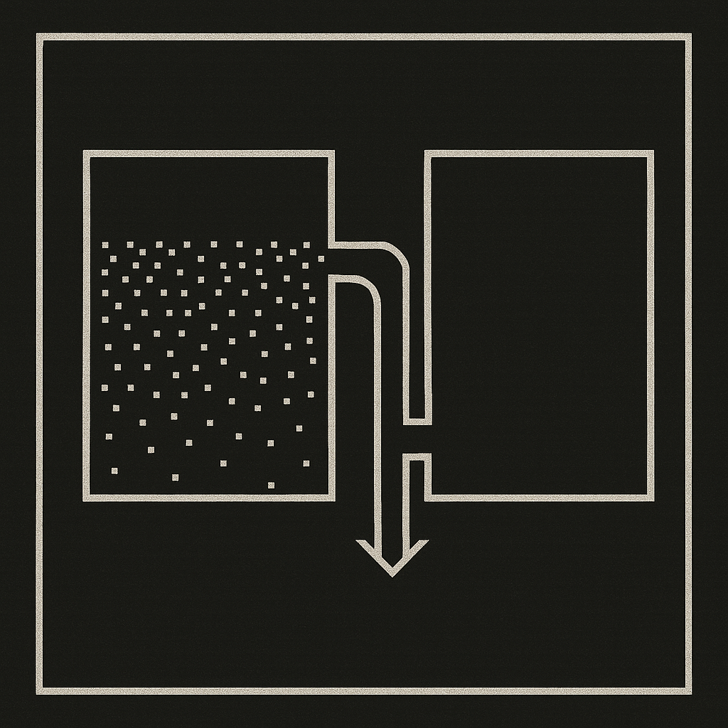
Nothing flows without a gradient.
Not heat. Not current. Not water. Not information. Not wealth. Not life.
Every river, every circuit, every living cell, every weather system, every economy runs on the same engine. A difference between two points. A slope in some quantity. An asymmetry that the universe cannot leave alone.
This document is the anatomy of that engine.
Nothing more.
What you do with it is your business.
PART ONE: THE UNIVERSAL ENGINE
Nothing Moves Without a Difference
Strip away the complexity of every system you have ever encountered. Every flowing river. Every beating heart. Every gust of wind. Every electrical circuit. Every chemical reaction.
Underneath all of them is one thing.
A difference.
Heat flows because one region is hotter than another. Current flows because one terminal has higher voltage than another. Water flows because one point has higher pressure than another. Molecules diffuse because one region has higher concentration than another.
Remove the difference and the flow stops. Instantly. Completely.
This is not a tendency. Not a preference. Not a statistical likelihood.
It is law.
    THE UNIVERSAL PRINCIPLE

    ┌────────────────────────────────────────────────────┐
    │                                                    │
    │    HIGH                              LOW           │
    │    ████████████  ──────────────►     ████           │
    │                                                    │
    │    Temperature, pressure, voltage,                 │
    │    concentration, elevation, wealth,               │
    │    information, chemical potential                  │
    │                                                    │
    │    Flow always runs from HIGH to LOW.              │
    │    Always. In every domain. No exceptions.         │
    │                                                    │
    └────────────────────────────────────────────────────┘
The gradient is the difference per unit distance. Not just that one end is hotter. How much hotter, per meter, per centimeter, per nanometer.
The steeper the gradient, the faster the flow.
The gentler the gradient, the slower the flow.
Zero gradient. Zero flow.
This is the first law of everything that moves.
What a Gradient Actually Is
The word comes from the Latin gradus. A step. A degree of change.
In mathematics, the gradient is a vector. It has magnitude and direction. Given any scalar field, any quantity distributed across space, the gradient points in the direction of steepest increase. Its magnitude tells you how steep that increase is.
    THE GRADIENT VECTOR

    Temperature field (°C):

        20°   25°   30°   35°   40°
         •─────•─────•─────•─────•

                    ────────────────►
                    Gradient direction
                    (toward steepest increase)

        Magnitude: 5°C per unit distance
        Direction: left to right

    Flux direction: ◄────────────────
    (opposite to gradient: high → low)
The gradient of a scalar field φ is written ∇φ.
The flux that results is proportional to the negative gradient. The negative sign matters. Flow runs downhill. Toward the lower value. Against the direction of steepest increase.
This single relationship generates almost every transport equation in physics.
PART TWO: THE THREE LAWS THAT ARE ONE LAW
The Deep Similarity
In the mid-1800s, three scientists working on three different problems discovered the same equation.
Jean-Baptiste Joseph Fourier studied heat. He found that heat flux is proportional to the negative temperature gradient.
Adolf Fick studied diffusion. He found that mass flux is proportional to the negative concentration gradient.
Georg Ohm studied electricity. He found that current density is proportional to the negative voltage gradient.
They thought they were describing different phenomena.
They were describing the same phenomenon.
    THE THREE LAWS THAT ARE ONE

    ┌────────────────────────────────────────────────────┐
    │                                                    │
    │  FOURIER'S LAW (1822)                              │
    │                                                    │
    │    Heat flux = -k × ∇T                             │
    │                                                    │
    │    k = thermal conductivity                        │
    │    T = temperature                                 │
    │    Flow: hot → cold                                │
    │                                                    │
    ├────────────────────────────────────────────────────┤
    │                                                    │
    │  FICK'S LAW (1855)                                 │
    │                                                    │
    │    Mass flux = -D × ∇C                             │
    │                                                    │
    │    D = diffusion coefficient                       │
    │    C = concentration                               │
    │    Flow: concentrated → dilute                     │
    │                                                    │
    ├────────────────────────────────────────────────────┤
    │                                                    │
    │  OHM'S LAW (1827)                                  │
    │                                                    │
    │    Current density = -σ × ∇V                       │
    │                                                    │
    │    σ = electrical conductivity                     │
    │    V = voltage                                     │
    │    Flow: high potential → low potential             │
    │                                                    │
    └────────────────────────────────────────────────────┘

    Same structure. Same sign. Same principle.

    Flux = -[conductivity] × ∇[potential]
Three domains. One architecture.
The medium changes. The quantity that flows changes. The conductivity coefficient changes.
The structure does not change.
Flux equals negative conductivity times gradient.
This is not coincidence. This is the universe revealing a single mechanism through three different windows.
The Linear Regime
Lars Onsager formalized this in 1931. He showed that near equilibrium, all transport phenomena obey the same linear relationship between forces and fluxes. Thermodynamic forces are gradients. Thermodynamic fluxes are the flows they produce.
When multiple gradients operate simultaneously, they can couple. A temperature gradient can drive mass flow. A concentration gradient can drive electrical current. A pressure gradient can drive heat transport.
Onsager proved that the coupling coefficients are symmetric. If a temperature gradient drives mass flow with strength L₁₂, then a concentration gradient drives heat flow with the same strength L₂₁.
    ONSAGER'S COUPLING MATRIX

    ┌──────────────────────────────────────────────┐
    │                                              │
    │   Flux₁ = L₁₁ × Force₁ + L₁₂ × Force₂      │
    │   Flux₂ = L₂₁ × Force₁ + L₂₂ × Force₂      │
    │                                              │
    │   L₁₂ = L₂₁  (Onsager reciprocity)          │
    │                                              │
    │   Direct effects:  L₁₁, L₂₂                 │
    │   Cross effects:   L₁₂ = L₂₁                │
    │                                              │
    │   The coupling is symmetric.                 │
    │   Nature does not play favorites             │
    │   between cause and effect.                  │
    │                                              │
    └──────────────────────────────────────────────┘
This won Onsager the Nobel Prize. Not for discovering a new force. For revealing a symmetry hidden inside the gradient.
PART THREE: THE ENGINE OF LIFE
The Proton Gradient
Life runs on a gradient.
Not metaphorically. Literally.
Every cell in your body manufactures ATP, the universal energy currency, by exploiting a proton gradient across a membrane. Peter Mitchell proposed this in 1961. It was so counterintuitive that the scientific community rejected it for over a decade.
He was right.
The electron transport chain pumps protons from one side of the mitochondrial inner membrane to the other. This creates two simultaneous gradients: a concentration gradient (more protons on one side) and an electrical gradient (positive charge accumulation on one side).
Together these form the proton motive force.
    THE CHEMIOSMOTIC ENGINE

                    OUTER SIDE (intermembrane space)
    ┌─────────────────────────────────────────────────┐
    │  H⁺  H⁺  H⁺  H⁺  H⁺  H⁺  H⁺  H⁺  H⁺  H⁺   │
    │  H⁺  H⁺  H⁺  H⁺  H⁺  H⁺  H⁺  H⁺  H⁺  H⁺   │
    │  HIGH concentration    HIGH positive charge     │
    └────────────────────┬────────────────────────────┘
                         │
              ══════╦════╧════╦══════  ← membrane
                    ║         ║
                    ║   ATP   ║
                    ║ SYNTHASE║
                    ║         ║
              ══════╩════╤════╩══════
                         │
    ┌────────────────────┴────────────────────────────┐
    │  H⁺        H⁺              H⁺                  │
    │       LOW concentration    LOW charge            │
    └─────────────────────────────────────────────────┘
                    INNER SIDE (matrix)

    Protons flow DOWN the gradient through ATP synthase.
    The flow physically rotates the enzyme.
    The rotation drives ADP + Pi → ATP.

    Gradient → mechanical rotation → chemical bond.
Protons flow down their gradient through ATP synthase. The flow literally rotates a molecular turbine. The rotation forces ADP and inorganic phosphate together to form ATP.
A gradient converts to mechanical rotation converts to chemical energy.
Your body synthesizes approximately 40 kilograms of ATP per day. Every molecule of it is manufactured by gradient flow.
The Morphogen Gradient
Development runs on gradients too.
A fertilized egg becomes a body because of concentration gradients of signaling molecules called morphogens. A morphogen is produced at a localized source, diffuses outward, and degrades as it spreads. The result is a smooth concentration gradient stretching away from the source.
Cells read their position by measuring the local morphogen concentration. High concentration means “near the source.” Low concentration means “far away.” Intermediate concentrations mean intermediate positions.
Different concentration thresholds activate different genes. The gradient becomes a coordinate system. Cells know where they are by what they can taste.
    MORPHOGEN GRADIENT IN DEVELOPMENT

    Concentration
         │
         │█
    HIGH │██
         │███
         │████
         │█████
         │██████
    MED  │████████
         │██████████
         │█████████████
         │████████████████
    LOW  │██████████████████████████████
         │
         └───────────────────────────────────────►
         Source                              Distance

    ┌──────────┐  ┌──────────┐  ┌──────────┐
    │  Gene A  │  │  Gene B  │  │  Gene C  │
    │  active  │  │  active  │  │  active  │
    │  (high)  │  │  (med)   │  │  (low)   │
    └──────────┘  └──────────┘  └──────────┘

    Position encoded in concentration.
    Identity encoded in threshold.
Sonic Hedgehog patterns the neural tube this way. Bicoid patterns the fruit fly anterior-posterior axis this way. Dozens of morphogens carve the body plan using nothing but diffusion, degradation, and threshold detection.
No blueprint. No master controller. Just gradients and thresholds.
PART FOUR: THE GRADIENT THAT DESTROYS ITSELF
The Second Law’s Demand
Here is the central paradox of gradient.
Every gradient drives a process. Every process the gradient drives diminishes the gradient.
Heat flows from hot to cold. The flow brings hot and cold closer together. The gradient flattens. Eventually, both regions reach the same temperature. Flow stops.
This is the Second Law of Thermodynamics expressed through gradient.
Entropy increases because gradients dissipate. Systems approach equilibrium because the flows they generate erode the differences that generate them.
    THE SELF-CONSUMING ENGINE

    TIME 0:
    ┌──────────────────────┐  ┌──────────────────────┐
    │                      │  │                      │
    │     100°C            │  │         0°C          │
    │     ████████████     │  │         ██           │
    │                      │  │                      │
    └──────────────────────┘  └──────────────────────┘
              Gradient: 100°C        Flow: FAST
                         │
                         ▼
    TIME 1:
    ┌──────────────────────┐  ┌──────────────────────┐
    │                      │  │                      │
    │      75°C            │  │        25°C          │
    │      █████████       │  │        █████         │
    │                      │  │                      │
    └──────────────────────┘  └──────────────────────┘
              Gradient: 50°C         Flow: MODERATE
                         │
                         ▼
    TIME 2:
    ┌──────────────────────┐  ┌──────────────────────┐
    │                      │  │                      │
    │      55°C            │  │        45°C          │
    │      ████████        │  │        ███████       │
    │                      │  │                      │
    └──────────────────────┘  └──────────────────────┘
              Gradient: 10°C         Flow: SLOW
                         │
                         ▼
    EQUILIBRIUM:
    ┌──────────────────────┐  ┌──────────────────────┐
    │                      │  │                      │
    │      50°C            │  │        50°C          │
    │      ███████         │  │        ███████       │
    │                      │  │                      │
    └──────────────────────┘  └──────────────────────┘
              Gradient: 0°C          Flow: ZERO
Every isolated system tends toward this fate. Maximum entropy. Zero gradient. No flow. No work. No process. No change.
The heat death of the universe is the final flattening of every gradient.
The Rate of Dying
The gradient does not die linearly. It dies exponentially.
The steeper the gradient, the faster the flow. The faster the flow, the faster the gradient erodes. Steep gradients destroy themselves quickly. Shallow gradients linger.
This produces exponential decay. The same curve that governs radioactive decay, capacitor discharge, Newton’s law of cooling, and the half-life of drugs in the bloodstream.
    EXPONENTIAL GRADIENT DECAY

    Gradient
    Magnitude
         │
         │█
    HIGH │██
         │████
         │██████
         │██████████
         │████████████████
    MED  │████████████████████████
         │████████████████████████████████
         │████████████████████████████████████████
    LOW  │████████████████████████████████████████████████████
         │
         └──────────────────────────────────────────────────►
                                                        Time

    Half-life: the time for the gradient to halve.
    Constant for a given system.
    Independent of starting magnitude.
The half-life depends on the conductivity of the medium and the geometry of the system. Copper dissipates electrical gradients in nanoseconds. Rock dissipates thermal gradients over millennia. But the curve is the same.
Every gradient is a clock. Counting down toward its own extinction.
PART FIVE: THE ENGINE OF STRUCTURE
How Gradients Build Order
Equilibrium is death. But the universe is not dead. Stars burn. Cells metabolize. Hurricanes spiral. Ecosystems cycle nutrients. Civilizations trade goods.
How does structure persist in a universe that relentlessly flattens every gradient?
By being fed.
Ilya Prigogine showed that when a system is held far from equilibrium by a sustained external gradient, new structures can spontaneously emerge. He called them dissipative structures. They exist because of the gradient, not despite it.
    DISSIPATIVE STRUCTURE FORMATION

    ┌──────────────────────────────────────────────┐
    │              EXTERNAL GRADIENT               │
    │         (sustained energy input)             │
    │                                              │
    │    Hot ██████████████████████████████ Cold    │
    │                                              │
    └──────────────────────┬───────────────────────┘
                           │
                           │ drives
                           ▼
    ┌──────────────────────────────────────────────┐
    │            SYSTEM FAR FROM                   │
    │              EQUILIBRIUM                     │
    │                                              │
    │    Random fluctuations amplify               │
    │    Symmetry breaks                           │
    │    Pattern crystallizes                      │
    │                                              │
    └──────────────────────┬───────────────────────┘
                           │
                           │ produces
                           ▼
    ┌──────────────────────────────────────────────┐
    │         ORGANIZED STRUCTURE                  │
    │         (dissipative structure)              │
    │                                              │
    │    Bénard convection cells                   │
    │    Chemical oscillations (BZ reaction)       │
    │    Hurricanes                                │
    │    Living organisms                          │
    │                                              │
    │    Structure dissipates the gradient         │
    │    MORE EFFICIENTLY than random flow         │
    │                                              │
    └──────────────────────────────────────────────┘
The Bénard experiment is the clearest demonstration. Heat a thin layer of fluid from below. A temperature gradient forms. Below a critical gradient, heat transfers by conduction alone. Random. Structureless. Inefficient.
Above the critical gradient, the fluid spontaneously organizes into hexagonal convection cells. Warm fluid rises in the center. Cool fluid sinks at the edges. A beautiful, ordered pattern emerges from nothing but a temperature difference.
The structure exists to dissipate the gradient faster. The universe does not care about order. It cares about flattening gradients. If organized flow dissipates a gradient more efficiently than random diffusion, organized flow wins.
Structure is gradient dissipation optimized.
Life as Gradient Exploitation
A living organism is a dissipative structure of extraordinary sophistication.
It maintains itself by channeling gradients. Chemical gradients across membranes drive ATP synthesis. Concentration gradients drive nutrient uptake. Electrochemical gradients drive neural signaling. Osmotic gradients drive water transport.
The organism does not fight the Second Law. It surfs it. It positions itself in the flow between high-potential energy sources and low-potential sinks, and it harvests the flow.
    LIFE AS GRADIENT CHANNELING

    ┌───────────────────┐
    │  HIGH POTENTIAL   │
    │  (sunlight, food, │
    │   chemical bonds) │
    └─────────┬─────────┘
              │
              │ gradient
              ▼
    ┌───────────────────┐
    │                   │
    │  LIVING ORGANISM  │
    │                   │
    │  Channels flow    │
    │  Extracts work    │
    │  Builds structure │
    │  Maintains self   │
    │                   │
    └─────────┬─────────┘
              │
              │ waste heat, entropy
              ▼
    ┌───────────────────┐
    │  LOW POTENTIAL    │
    │  (heat, CO₂,     │
    │   disorder)       │
    └───────────────────┘

    Death = loss of gradient access.
    Not loss of matter. Not loss of structure.
    Loss of flow.
When the gradient stops, the organism stops. Not because it runs out of material. Because it runs out of difference. A dead body has the same atoms as a living one. It has lost access to the gradient.
Death is gradient disconnection.
PART SIX: THE LANDSCAPE
Gradient Descent
Every optimization process in nature and mathematics follows gradients downhill.
A ball rolls to the bottom of a valley. Water finds the lowest path. A chemical reaction proceeds toward minimum free energy. A neural network adjusts its weights to minimize loss.
The principle is the same. Measure the gradient of the function you want to minimize. Take a step in the opposite direction. Repeat.
    GRADIENT DESCENT ON A LOSS LANDSCAPE

    Loss
         │
         │    ·
    HIGH │  ·   ·
         │ ·     ·
         │·       ·              ·
         │         ·           ·   ·
    MED  │          ·        ·       ·
         │           ·     ·          ·
         │            ·  ·             ·
    LOW  │             ··               ·····
         │              ▲
         └──────────────┼──────────────────────►
                        │                 Parameter
                   Global
                   minimum

    At each point, the gradient tells you:
    - Which direction is downhill (direction)
    - How steep the slope is (magnitude)

    Step size = learning rate × gradient magnitude
In machine learning, this is made explicit. The loss function defines a landscape. The gradient of the loss with respect to each parameter tells the algorithm which way to adjust. Steeper gradient means larger adjustment. Flat gradient means the algorithm has found a valley.
But the landscape is not smooth. It has local minima, saddle points, plateaus. Places where the gradient vanishes but the position is not optimal. The system gets trapped. Not because it stopped following the gradient. Because the gradient stopped pointing anywhere useful.
This is the fundamental limitation of gradient following. It is greedy. It sees only the local slope. It cannot see the global landscape.
Saddle Points and Flat Regions
In high-dimensional spaces, true local minima are rare. Most critical points where the gradient vanishes are saddle points. The landscape curves downward in some directions and upward in others.
    CRITICAL POINTS IN OPTIMIZATION

    ┌──────────────────────────────────────────────┐
    │                                              │
    │  LOCAL MINIMUM        SADDLE POINT           │
    │                                              │
    │      \    /              \    ↗              │
    │       \  /                \  /               │
    │        \/                  \/                 │
    │                            /\                │
    │  Gradient = 0             /  \               │
    │  Curves up in ALL        Gradient = 0        │
    │  directions              Curves up in SOME   │
    │  (trapped)               Curves down in      │
    │                          others (escapable)  │
    │                                              │
    ├──────────────────────────────────────────────┤
    │                                              │
    │  PLATEAU                 GLOBAL MINIMUM      │
    │                                              │
    │  ─────────────              \      /         │
    │                              \    /          │
    │  Gradient ≈ 0                 \  /           │
    │  Nearly flat                   \/            │
    │  (slow progress)                             │
    │                          Gradient = 0        │
    │                          Lowest possible     │
    │                          (optimal)           │
    │                                              │
    └──────────────────────────────────────────────┘
The noise in stochastic gradient descent is not a flaw. It is an escape mechanism. The random perturbations jostle the system out of shallow traps and across saddle points. Too much noise and the system never settles. Too little and it gets stuck in the first valley it finds.
The optimal amount of noise depends on the landscape. And the landscape is never known in advance.
PART SEVEN: THE SOCIAL GRADIENT
Wealth, Power, and Information
Gradients operate in social systems with the same structural logic as in physical ones.
Wealth flows. Not randomly. Down gradients of opportunity and up gradients of extraction. When a large wealth differential exists between two connected populations, resources flow toward the population with more leverage, more infrastructure, more ability to capture value.
The pattern mirrors fluid dynamics. Steeper wealth gradients produce faster flows. The flows can go either direction depending on the institutional channels through which they run.
    GRADIENT FLOWS IN SOCIAL SYSTEMS

    PHYSICAL SYSTEM              SOCIAL SYSTEM

    Temperature gradient    →    Wealth gradient
    Heat flux               →    Capital flow
    Conductivity            →    Institutional access
    Insulation              →    Barriers to entry

    Pressure gradient       →    Power gradient
    Fluid flow              →    Influence flow
    Viscosity               →    Social friction

    Concentration gradient  →    Information gradient
    Diffusion               →    Information spread
    Membrane permeability   →    Access to networks
Information asymmetry is a gradient. One party knows something the other does not. The gradient creates an advantage. Markets, negotiations, political systems, and hierarchies all operate on information gradients.
The efficient market hypothesis claims that information gradients in financial markets flatten almost instantly. New information diffuses through the network of traders until everyone knows the same thing and the gradient disappears.
In practice, information gradients persist. Insider knowledge. Proprietary data. Classified intelligence. Asymmetric expertise. These are maintained gradients. They persist because barriers prevent the natural diffusion that would flatten them.
Power is a maintained gradient. It requires continuous energy input to sustain. The moment the maintenance stops, the gradient begins to flatten. Hierarchies that stop reinforcing themselves dissolve.
Network Gradients
In network theory, centrality is a gradient. Some nodes have many connections. Most have few. The distribution follows a power law in scale-free networks.
The gradient between central and peripheral nodes determines the flow of information, influence, and resources through the network. Central nodes see more, faster. Peripheral nodes see less, slower.
    NETWORK CENTRALITY GRADIENT

    ┌──────────────────────────────────────────────┐
    │                                              │
    │              ┌───┐                           │
    │         ┌────┤ A ├────┐                      │
    │         │    └─┬─┘    │                      │
    │      ┌──┴──┐   │   ┌──┴──┐                   │
    │      │  B  │   │   │  C  │                   │
    │      └──┬──┘   │   └──┬──┘                   │
    │         │    ┌─┴─┐    │                      │
    │         └────┤ D ├────┘                      │
    │              └─┬─┘                           │
    │                │                             │
    │             ┌──┴──┐                          │
    │             │  E  │                          │
    │             └─────┘                          │
    │                                              │
    │  Centrality:  A,D > B,C > E                  │
    │  Information reaches A and D first.          │
    │  E learns last. Always.                      │
    │                                              │
    └──────────────────────────────────────────────┘
The gradient is not just descriptive. It is generative. The centrality gradient creates preferential attachment. New connections form preferentially to already-central nodes. The rich get richer. The gradient steepens itself.
Until a disruption occurs. A new technology. A new network topology. A revolution. These events flatten one gradient and create another.
PART EIGHT: THE MAINTENANCE PROBLEM
Sustained Gradients Require Work
Every gradient in the universe is either being maintained or dissipating.
There is no third option.
A battery maintains a voltage gradient by converting chemical energy. A heart maintains a pressure gradient by converting ATP. The sun maintains a temperature gradient by converting nuclear binding energy. A company maintains a competitive gradient by converting labor and capital.
    GRADIENT MAINTENANCE

    ┌──────────────────────────────────────────────────┐
    │                                                  │
    │  SUSTAINED GRADIENT = CONTINUOUS ENERGY INPUT    │
    │                                                  │
    │  Battery         Chemical energy → Voltage       │
    │  Heart           ATP → Pressure                  │
    │  Sun             Nuclear fusion → Temperature    │
    │  Cell membrane   ATP → Ion concentration         │
    │  Refrigerator    Electricity → Temperature       │
    │  Organization    Labor/capital → Competitive     │
    │                  advantage                       │
    │                                                  │
    │  Remove the input. Watch the gradient die.       │
    │                                                  │
    └──────────────────────────────────────────────────┘
The refrigerator is the clearest example. It maintains a temperature gradient between inside and outside. It does this by pumping heat out, consuming electrical energy. Unplug it. The gradient begins to dissipate immediately. The inside warms. The outside cools by an immeasurable amount. Eventually both reach room temperature.
The gradient was never a thing. It was a process. A continuously maintained departure from equilibrium.
Every interesting system in the universe is a continuously maintained departure from equilibrium.
The Cost of Maintenance
Maintaining a gradient always costs more energy than the gradient contains.
This is the Second Law in economic terms. You cannot break even. The refrigerator consumes more energy than it would take to cool the food by other means. The cell spends more ATP maintaining its ion gradients than those gradients can recover. The organization burns more resources maintaining its market position than the position returns in any single transaction.
The maintenance is worth it because the gradient enables work. The ion gradient enables neural signaling. The market position enables revenue. The voltage gradient enables computation.
The gradient is not the product. The gradient is the engine. The work it enables is the product.
    THE ECONOMICS OF GRADIENT

    ┌──────────────────────────────────────────────────┐
    │                                                  │
    │   Energy to          Energy the         Value of │
    │   maintain    >      gradient    <      the work │
    │   gradient           contains           enabled  │
    │                                                  │
    │   Cost > Stored energy < Output value            │
    │                                                  │
    │   The gradient is NEVER the end product.         │
    │   It is always the MEANS.                        │
    │                                                  │
    │   You maintain the gradient because of           │
    │   what flows THROUGH it.                         │
    │                                                  │
    └──────────────────────────────────────────────────┘
PART NINE: THE CONSTRAINTS
The Steepness Limit
Gradients cannot be infinitely steep. Every medium has a maximum gradient it can sustain before the system breaks.
Electrical insulation breaks down above a critical voltage gradient. The dielectric strength is the maximum electric field a material can withstand before current punches through. Air breaks down at about 3 million volts per meter. That is lightning.
Thermal gradients cause mechanical stress. A steep temperature gradient in a solid creates differential expansion. If the gradient is too steep, the material cracks. Thermal shock.
Concentration gradients drive osmotic pressure. If the gradient across a cell membrane is too steep, the osmotic pressure ruptures the cell. Lysis.
    GRADIENT FAILURE MODES

    Gradient
    Steepness
         │
         │                    ┌─────────────────┐
    MAX  │  ─ ─ ─ ─ ─ ─ ─ ─ ─│   BREAKDOWN      │
         │                    │   System fails   │
         │                    │   Lightning      │
         │                    │   Fracture       │
         │                    │   Rupture        │
         │                    └─────────────────┘
         │
    HIGH │    ████████████████████
         │    Functional but stressed
         │
    MED  │    ████████████████
         │    Optimal operating range
         │
    LOW  │    ██████████
         │    Functional but slow
         │
         └──────────────────────────────────────────►
                                              Time
Every system has an operating range. Too shallow a gradient and nothing flows fast enough. Too steep and the medium fails. The useful gradient lives in the band between stagnation and destruction.
The Coupling Constraint
When multiple gradients operate in the same system, they interact. A temperature gradient can drive mass flow (thermodiffusion). A concentration gradient can drive electrical current (electroosmosis). A pressure gradient can drive heat transport (mechanocaloric effect).
These couplings are unavoidable. You cannot create a gradient in one quantity without disturbing others.
This means that optimizing one gradient often degrades another. A steeper chemical gradient in a battery increases power output but accelerates degradation. A steeper pressure gradient in a pipe increases flow but increases turbulence and friction losses.
    GRADIENT COUPLING

                GRADIENT A
                    │
         ┌──────────┼──────────┐
         │          │          │
         ▼          ▼          ▼
    ┌─────────┐ ┌─────────┐ ┌─────────┐
    │ Flux A  │ │ Flux B  │ │ Flux C  │
    │ (wanted)│ │ (cross) │ │ (cross) │
    │         │ │         │ │         │
    │ Direct  │ │Unwanted │ │Unwanted │
    │ effect  │ │coupling │ │coupling │
    └─────────┘ └─────────┘ └─────────┘

    You cannot drive Flux A without also
    producing Flux B and Flux C.

    Engineering is the art of maximizing
    direct effects and minimizing cross effects.
Engineering is not the creation of gradients. It is the management of their couplings. The discipline of maximizing the useful flow while minimizing the parasitic ones.
The Direction Constraint
Gradients impose directionality. Flow runs downhill. Always. You cannot make heat flow from cold to hot without doing work. You cannot make molecules diffuse from low concentration to high without energy input.
This directionality is the arrow of time itself.
The Second Law of Thermodynamics says that the total entropy of an isolated system never decreases. This is equivalent to saying that net flow always runs down the gradient. Local reversals are possible. You can pump heat uphill. But the pump consumes energy and creates more entropy elsewhere than it reduces locally.
The global gradient always flattens. The global arrow always points toward equilibrium.
PART TEN: ENTROPY PRODUCTION AND THE GRADIENT
The Rate of Entropy
Entropy production is proportional to flux times gradient.
This is the central equation of irreversible thermodynamics. It tells you exactly how fast a system generates entropy. How fast it moves toward equilibrium. How fast it ages.
    ENTROPY PRODUCTION

    σ = Σ (Flux_i × Force_i)

    ┌──────────────────────────────────────────────────┐
    │                                                  │
    │  Entropy production = sum of all                 │
    │  (flow × driving gradient) pairs                 │
    │                                                  │
    │  Heat conduction:   σ = q × ∇(1/T)              │
    │  Diffusion:         σ = J × ∇(-μ/T)             │
    │  Viscous flow:      σ = τ × ∇v                   │
    │                                                  │
    │  Larger flux = faster entropy production         │
    │  Larger gradient = faster entropy production     │
    │  Both together = maximum aging rate              │
    │                                                  │
    └──────────────────────────────────────────────────┘
A steep gradient and a conductive medium produce maximum entropy. The system ages fastest. Equilibrium arrives soonest.
A gentle gradient and a resistive medium produce minimum entropy. The system ages slowly. The gradient persists longer.
Nature selects for both. When dissipation serves a purpose (cooling, transport, signaling), steep gradients and conductive media win. When preservation serves a purpose (insulation, storage, protection), gentle gradients and resistive media win.
The choice is never whether to produce entropy. It is always how fast, and in service of what.
PART ELEVEN: THE COMPLETE PICTURE
The Unified Framework
Everything connects.
    THE COMPLETE GRADIENT FRAMEWORK

    ┌─────────────────────────────────────────────────────────┐
    │                                                         │
    │                    THE GRADIENT                         │
    │                                                         │
    │    A difference in a quantity distributed across         │
    │    space or across a boundary. The universal             │
    │    engine of all flow, all work, all structure.         │
    │                                                         │
    └─────────────────────────────────────────────────────────┘
                              │
              ┌───────────────┼───────────────┐
              │               │               │
              ▼               ▼               ▼
    ┌─────────────────┐ ┌─────────────┐ ┌─────────────────┐
    │                 │ │             │ │                 │
    │  TRANSPORT      │ │  STRUCTURE  │ │  OPTIMIZATION   │
    │                 │ │             │ │                 │
    │  Fourier, Fick, │ │ Dissipative │ │  Gradient       │
    │  Ohm, Darcy     │ │ structures  │ │  descent        │
    │                 │ │ Life        │ │  Natural        │
    │  Flux = -k∇φ    │ │ Hurricanes  │ │  selection      │
    │                 │ │ Economies   │ │  Learning       │
    │                 │ │             │ │                 │
    └─────────────────┘ └─────────────┘ └─────────────────┘
              │               │               │
              └───────────────┼───────────────┘
                              │
                              ▼
    ┌─────────────────────────────────────────────────────────┐
    │                                                         │
    │                 THE CONSTRAINT                          │
    │                                                         │
    │    Every gradient consumes itself through the flow      │
    │    it generates. Sustained gradient requires            │
    │    sustained energy input. No input, no gradient.       │
    │    No gradient, no flow. No flow, no structure.         │
    │    No structure, equilibrium. Heat death.               │
    │                                                         │
    └─────────────────────────────────────────────────────────┘
The gradient is the most fundamental engine in the universe.
Not because it is complex. Because it is simple. A difference between two points. Nothing more.
From this difference: rivers. Circuits. Cells. Brains. Economies. Weather. Stars.
From the erasure of this difference: entropy. Equilibrium. Death.
The Operating Principles
    THE LAWS OF GRADIENT

    ┌─────────────────────────────────────────────────────────┐
    │                                                         │
    │   PRINCIPLE 1: NO GRADIENT, NO FLOW                     │
    │                                                         │
    │   Nothing moves without a difference.                   │
    │   Equilibrium is absolute stillness.                    │
    │                                                         │
    └─────────────────────────────────────────────────────────┘

    ┌─────────────────────────────────────────────────────────┐
    │                                                         │
    │   PRINCIPLE 2: FLOW DESTROYS GRADIENT                   │
    │                                                         │
    │   Every process a gradient drives erodes                │
    │   the gradient that drives it. Exponentially.           │
    │                                                         │
    └─────────────────────────────────────────────────────────┘

    ┌─────────────────────────────────────────────────────────┐
    │                                                         │
    │   PRINCIPLE 3: SUSTAINED GRADIENT REQUIRES WORK         │
    │                                                         │
    │   The only way to maintain a gradient is to             │
    │   feed it continuously. The cost always exceeds         │
    │   the stored energy.                                    │
    │                                                         │
    └─────────────────────────────────────────────────────────┘

    ┌─────────────────────────────────────────────────────────┐
    │                                                         │
    │   PRINCIPLE 4: STRUCTURE IS GRADIENT DISSIPATION        │
    │                                                         │
    │   Organized patterns emerge because they                │
    │   dissipate gradients more efficiently than             │
    │   random diffusion.                                     │
    │                                                         │
    └─────────────────────────────────────────────────────────┘

    ┌─────────────────────────────────────────────────────────┐
    │                                                         │
    │   PRINCIPLE 5: EVERY GRADIENT HAS A BREAKING POINT     │
    │                                                         │
    │   Too steep and the medium fails. Lightning.            │
    │   Fracture. Rupture. Revolution.                        │
    │                                                         │
    └─────────────────────────────────────────────────────────┘
Final Synthesis
The universe runs on difference.
Not on things. Not on substances. Not on particles or waves or fields in themselves.
On the gaps between them.
The gap between hot and cold moves heat. The gap between high pressure and low pressure moves air. The gap between concentrated and dilute moves molecules. The gap between high potential and low potential moves charge.
Close the gap and nothing happens. Open the gap and everything happens.
A gradient is not a thing. It is a relationship. A slope. A tilt in the landscape of some quantity. And it is this tilt, not the quantity itself, that generates every phenomenon worth studying.
Life is gradient exploitation. Death is gradient loss. Structure is gradient dissipation organized. Equilibrium is gradient extinction.
The cell membrane that keeps sodium outside and potassium inside. The atmosphere that keeps the tropics warm and the poles cold. The economy that keeps capital concentrated in nodes of high return. The star that keeps its core at 15 million degrees while its surface radiates at 5,800.
All of them are the same machinery.
A difference, maintained against the tide of entropy, driving a flow, enabling a process, producing something the universe would not produce at equilibrium.
The gradient does not care what flows through it. Heat, charge, mass, information, influence, capital. The engine is indifferent to its cargo. It only asks one question.
Is there a difference?
If yes: flow.
If no: nothing.
That is the complete machinery of gradient.
CITATIONS
Foundational Transport Theory
Fourier’s Law and Heat Conduction
Fourier, J.B.J. (1822). Théorie analytique de la chaleur. Firmin Didot, Paris.
Fick’s Laws of Diffusion
Fick, A. (1855). “Ueber Diffusion.” Annalen der Physik, 170(1):59-86. https://en.wikipedia.org/wiki/Fick%27s_laws_of_diffusion
Revised Formulation of Transport Laws
Won, Y.-Y. et al. (2019). “Revised Formulation of Fick’s, Fourier’s, and Newton’s Laws for Spatially Varying Linear Transport Coefficients.” ACS Omega, 4(6):11215-11222. PMC6648224. https://pmc.ncbi.nlm.nih.gov/articles/PMC6648224/
Non-Equilibrium Thermodynamics
Onsager Reciprocal Relations
Onsager, L. (1931). “Reciprocal Relations in Irreversible Processes.” Physical Review, 37(4):405-426.
Gradient Dynamics and Entropy Production
Mielke, A. (2017). “Gradient Dynamics and Entropy Production Maximization.” Journal of Non-Equilibrium Thermodynamics, 42(4). https://www.degruyterbrill.com/document/doi/10.1515/jnet-2017-0005/html
Non-Equilibrium Thermodynamics in Biological Systems
Gnesotto, F.S. et al. (2018). “Broken detailed balance and non-equilibrium dynamics in living systems: a review.” Reports on Progress in Physics, 81(6):066601. https://par.nsf.gov/servlets/purl/10170794
Dissipative Structures and Self-Organization
Prigogine’s Framework
Prigogine, I. & Nicolis, G. (1977). Self-Organization in Nonequilibrium Systems. Wiley.
Thermodynamics of Self-Organization
Kondepudi, D.K. et al. (2020). “On the Thermodynamics of Self-Organization in Dissipative Systems.” Entropy. https://par.nsf.gov/servlets/purl/10356620
Dissipative Structures in Evolution
Brooks, D.R. & Wiley, E.O. (1988). “Applying the Prigogine view of dissipative systems to the major transitions in evolution.” Paleobiology. https://www.cambridge.org/core/journals/paleobiology/article/applying-the-prigogine-view-of-dissipative-systems-to-the-major-transitions-in-evolution/950CC803571570A46EEF7EE5970C50A1
Biological Gradients
Chemiosmotic Hypothesis
Mitchell, P. (1961). “Coupling of phosphorylation to electron and hydrogen transfer by a chemi-osmotic type of mechanism.” Nature, 191(4784):144-148.
Morphogen Gradients
Kicheva, A. et al. (2022). “Precision of morphogen gradients in neural tube development.” Nature Communications, 13:1145. https://www.nature.com/articles/s41467-022-28834-3
Morphogen Patterning Principles
Stapornwongkul, K.S. & Vincent, J.-P. (2022). “Patterning principles of morphogen gradients.” Open Biology, 12(10):220224. https://royalsocietypublishing.org/rsob/article/12/10/220224/91148/Patterning-principles-of-morphogen
Biomolecular Gradients
Wikipedia contributors. “Biomolecular gradient.” Wikipedia. https://en.wikipedia.org/wiki/Biomolecular_gradient
Gradient Descent and Optimization
Loss Landscape Geometry
Qu, Z. et al. (2025). “Optimization on multifractal loss landscapes explains a diverse range of geometrical and dynamical properties of deep learning.” Nature Communications, 16:4265. https://www.nature.com/articles/s41467-025-58532-9
Gradient Flow as Navigation
Tyulmankov, D. et al. (2025). “Gradient Descent as Loss Landscape Navigation.” arXiv:2510.26997. https://arxiv.org/pdf/2510.26997
Social and Network Gradients
Network Centrality and Inequality
Hanneman, R.A. & Riddle, M. “Introduction to social network methods: Chapter 10: Centrality and power.” https://faculty.ucr.edu/~hanneman/nettext/C10_Centrality.html
Emergent Inequality in Networks
Boghosian, B.M. et al. (2017). “Emergent inequality and self-organized social classes in a network of power and frustration.” PLoS ONE. PMC5315399. https://www.ncbi.nlm.nih.gov/pmc/articles/PMC5315399/
Social Hierarchies and Networks
Hobson, E.A. et al. (2022). “Social hierarchies and social networks in humans.” Philosophical Transactions of the Royal Society B, 377(1845):20200440. https://royalsocietypublishing.org/rstb/article/377/1845/20200440/108822/Social-hierarchies-and-social-networks-in
Pressure Gradients and Fluid Dynamics
Atmospheric Pressure Gradients
University Corporation for Atmospheric Research. “Pressure Gradient Force Explained.” https://au1.ucar.edu/what-is-a-pressure-gradient-force
Pressure Gradients in Fluid Dynamics
Elsevier. “Pressure Gradients in Fluid Dynamics.” https://elsevier.blog/pressure-gradients-fluid-dynamics/
Document compiled from foundational physics, thermodynamics, biochemistry, network theory, and optimization theory. All transport phenomena unified under the gradient principle.
Related Machineries
- THE MACHINERY OF ENTROPY. Entropy is what happens when gradients dissipate. The entropy guide’s central thesis is that structure emerges to dissipate gradients faster.
- THE MACHINERY OF EQUILIBRIUM. Equilibrium is the gradient-exhausted state. Zero gradient, zero flow, zero change. The endpoint this guide’s engine is always approaching.
- THE MACHINERY OF DECAY. Decay is gradient dissipation measured in time. The exponential curve that governs every gradient’s decline is the same curve that governs every form of decay.