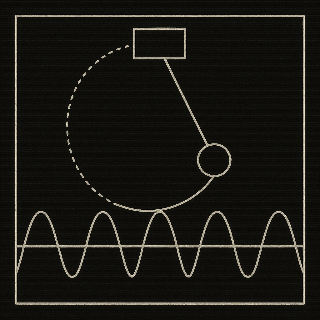
THE MACHINERY OF CYCLES
A Complete Guide to Periodic Return
How the Architecture of Recurrence Actually Works
What follows is not advice.
It is not a metaphor for seasons. Not a productivity framework about rhythms. Not another circular diagram about life stages.
It is mechanism.
The actual mathematics of why systems return. The physics of oscillation. The structural conditions that make periodicity inevitable and the conditions that destroy it.
Most people use the word “cycle” as decoration. They say things cycle. Markets cycle. Moods cycle. Relationships cycle. But they never ask the real question.
Why does anything return at all?
A ball thrown forward does not come back. A river flowing downhill does not climb. In a universe governed by thermodynamic dissipation, the default trajectory is one-way. Decay. Dispersal. Equilibrium.
And yet cycles are everywhere. Orbits. Heartbeats. Chemical oscillations. Ice ages. Population booms and collapses. Economic expansions and contractions. The cell dividing. The pendulum swinging. The predator chasing the prey that feeds the predator.
Return is not the default. Return requires structure.
This document is about that structure.
PART ONE: THE ANATOMY OF RETURN
What a Cycle Actually Is
A cycle is a trajectory in state space that closes on itself.
That sentence contains everything. But it needs unpacking.
Every system has a state. The state is the complete description of the system at a single moment. For a pendulum, the state is its angle and angular velocity. For a population, the state is the number of organisms. For a chemical reaction, the state is the concentration of each species.
The space of all possible states is called phase space. Every point in phase space is a possible configuration of the system. As the system evolves, it traces a path through this space.
A cycle is a path that returns to where it started.
    PHASE SPACE TRAJECTORY

    State
    Variable B
         │
         │         ┌──────────────┐
         │        /                \
         │       /                  \
         │      │                    │
         │      │     CYCLE          │
         │      │   (closed orbit)   │
         │       \                  /
         │        \                /
         │         └──────────────┘
         │
         └──────────────────────────────────────────►
                   State Variable A


    ONE-WAY TRAJECTORY (no cycle):

         │
         │   •
         │    \
         │     \
         │      •───────────•──────────►
         │
         └──────────────────────────────────────────►
The one-way trajectory reaches a point and stays. That point is a fixed point. An equilibrium. The system settles and nothing changes.
The closed orbit never settles. It returns, and returns, and returns.
The question is not whether cycles exist. They obviously do. The question is what structure forces a trajectory to close on itself rather than collapse to a point.
The Period and the Phase
Every cycle has two fundamental properties.
The period is how long one complete traversal takes. The period of Earth’s orbit is one year. The period of a heartbeat is roughly one second. The period of a Kondratiev economic wave is roughly fifty years.
The phase is where on the cycle the system currently sits. Two systems can have identical cycles but different phases. They trace the same path but at different positions along it.
    PERIOD AND PHASE

    Value
      │
      │    ┌─┐           ┌─┐           ┌─┐
      │   /   \         /   \         /   \
      │  /     \       /     \       /     \
      │ /       \     /       \     /       \
    ──┼/─────────\───/─────────\───/─────────\──────►
      │           \ /           \ /           \    Time
      │            V             V             V
      │
      │   ◄───────────►
      │      PERIOD T
      │
      │           ▲
      │           │
      │         PHASE
      │    (position on cycle
      │     at time t)
Period tells you the timescale of return. Phase tells you the current position. Together they define the cycle completely.
But neither tells you why the cycle exists.
PART TWO: THE GENERATOR
The Recipe for Oscillation
Cycles do not appear spontaneously. They require a specific structural recipe.
Two ingredients. Both necessary. Neither sufficient alone.
Ingredient one: negative feedback.
A mechanism that pushes the system back toward some reference. Gravity pulls the pendulum back toward vertical. Predator growth reduces prey. Price increases reduce demand.
Negative feedback alone produces no cycle. It produces a return to equilibrium. A direct, monotonic collapse to the center. Overshoot is impossible because the correction is instantaneous.
Ingredient two: delay.
A gap between the cause and the correction. The pendulum has momentum. It does not stop at vertical. It carries past. The predator population does not decline the instant prey becomes scarce. It takes time for starvation to reduce numbers. The market does not correct instantly. Information takes time to propagate.
Delay means the correction arrives after the system has already moved too far.
    THE OSCILLATION GENERATOR

    ┌──────────────────────────────────────────────────────┐
    │                                                      │
    │   NEGATIVE FEEDBACK             DELAY                │
    │   (restoring force)      +      (temporal gap)       │
    │                                                      │
    │              │                      │                │
    │              └──────────┬───────────┘                │
    │                         │                            │
    │                         ▼                            │
    │                                                      │
    │                    OVERSHOOT                          │
    │                                                      │
    │          System passes the target.                    │
    │          Correction arrives late.                     │
    │          Pushes past the other side.                  │
    │          Correction arrives late again.               │
    │                                                      │
    │                    = CYCLE                            │
    │                                                      │
    └──────────────────────────────────────────────────────┘
This is the universal generator. Every sustained oscillation in nature traces back to this structure. Delayed negative feedback.
The pendulum swings through the center because momentum creates delay. The predator overshoots because reproduction lag creates delay. The economy overheats because investment commitment creates delay. The thermostat oscillates because thermal inertia creates delay.
No delay, no overshoot. No overshoot, no cycle.
Damping and Driving
Not every oscillation lasts.
The pendulum slows. Air resistance removes energy on each swing. The amplitude shrinks. The cycle spirals inward toward the fixed point.
This is a damped oscillation. The cycle exists as a transient. It appears, it decays, it dies.
    DAMPED VS SUSTAINED OSCILLATION

    DAMPED:
    Value
      │   /\      /\
      │  /  \    /  \    /\
      │ /    \  /    \  /  \_____________________
    ──┼/──────\/──────\/─────────────────────────►
      │                                        Time
      │   (amplitude decays to zero)


    SUSTAINED:
    Value
      │   /\    /\    /\    /\    /\    /\
      │  /  \  /  \  /  \  /  \  /  \  /  \
    ──┼/────\/────\/────\/────\/────\/────\/──►
      │                                    Time
      │   (amplitude remains constant)
For a cycle to persist, something must replace the energy that dissipation removes.
The clock pendulum has an escapement mechanism. A small kick on every swing, timed precisely to offset friction. The heart has pacemaker cells. A biochemical pulse that re-fires the contraction. The Belousov-Zhabotinsky reaction has autocatalysis. A chemical pathway that regenerates its own reactants.
A sustained cycle requires an energy source coupled to the oscillation.
Without the source, every cycle is temporary.
With the source, the cycle becomes self-sustaining.
This self-sustaining oscillation has a name in mathematics. It is called a limit cycle.
PART THREE: THE LIMIT CYCLE
Poincaré’s Isolated Orbit
Henri Poincaré introduced the concept in the 1880s while studying celestial mechanics.
A limit cycle is a closed orbit in phase space that is isolated. Isolated means it is not surrounded by other closed orbits. It stands alone. Nearby trajectories either spiral toward it or away from it.
A stable limit cycle attracts. Start anywhere near it, and the system spirals inward until it locks onto the orbit. The amplitude and frequency are determined by the structure of the system, not by where you started.
This is the critical distinction.
A simple harmonic oscillator has a family of orbits. Every amplitude is possible. Push the pendulum harder, it swings wider. The orbit depends on initial conditions.
A limit cycle has one orbit. One amplitude. One frequency. Regardless of where you begin. Push it harder, it returns to the same amplitude. Perturb it, it recovers. The cycle is an attractor.
    LIMIT CYCLE AS ATTRACTOR

    State B
         │
         │   \  ╲               ╱  /
         │    \  ╲    ┌────┐   ╱  /
         │     \  ╲  /      \ ╱  /
         │      ╲  ╲/        ╱  /
         │       ╲  │ LIMIT │ ╱
         │        ╲ │ CYCLE │╱
         │         ╲\      /╱
         │          ╲└────┘╱
         │           ╱    ╲
         │          ╱      ╲
         │
         └──────────────────────────────────────────►
                   State A

    All nearby trajectories spiral
    TOWARD the closed orbit.

    Start inside → spiral outward to it.
    Start outside → spiral inward to it.
    The cycle itself is the attractor.
The heartbeat is a limit cycle. Perturb it and it returns to roughly the same rhythm. The circadian clock is a limit cycle. Jet lag is the transient spiral back to the attractor after displacement. The Belousov-Zhabotinsky reaction is a limit cycle. Dilute it or concentrate it and the oscillation re-establishes at the same frequency.
Limit cycles are the mathematical objects behind every self-sustaining rhythm in nature.
The Poincaré-Bendixson Theorem
In two-dimensional phase spaces, there is a remarkable theorem.
If a trajectory is confined to a bounded region and cannot reach a fixed point, it must approach a limit cycle.
The trajectory has nowhere else to go. It cannot leave the region. It cannot settle to a point. The only remaining option is periodic orbit.
This means that in two-dimensional systems, the alternatives are stark. Equilibrium or oscillation. Stasis or cycle. There is no third option.
In three or more dimensions, a third option appears. Chaos. Trajectories that never repeat, never settle, never close. But in two dimensions, the Poincaré-Bendixson theorem forbids chaos.
Confined motion that cannot rest must cycle.
PART FOUR: THE THERMODYNAMIC ENGINE
Work Requires Cycling
A heat engine extracts work from a temperature difference.
But it cannot do this in a single step. It must cycle. The working fluid must return to its initial state so the process can repeat.
This is Sadi Carnot’s insight from 1824. The most efficient possible engine operates in a cycle of four steps. Two isothermal. Two adiabatic. The fluid expands at the hot temperature, absorbing heat. It expands further without heat exchange. It compresses at the cold temperature, rejecting heat. It compresses further back to the start.
    THE CARNOT CYCLE IN P-V SPACE

    Pressure
         │
         │  A
         │  ●────────────────●  B
         │  │   isothermal    \
         │  │   expansion      \  adiabatic
         │  │   (absorb heat)   \  expansion
         │  │                    \
         │  │                     ●  C
         │  │    ┌─── WORK ───┐   │
         │  │    │  EXTRACTED  │   │  isothermal
         │  │    └─────────────┘   │  compression
         │  │                     /   (reject heat)
         │  │                    /
         │  │                   ●  D
         │  │                  /
         │  │   adiabatic     /
         │  │   compression  /
         │  ●───────────────●
         │  A
         │
         └──────────────────────────────────────────►
                       Volume
The area enclosed by the cycle in pressure-volume space equals the net work extracted.
No cycle, no enclosed area. No enclosed area, no net work.
A system that simply expands does work once and stops. A system that cycles does work repeatedly. The cycle is not incidental to the engine. The cycle is the engine.
The Efficiency Bound
Carnot proved that no engine operating between temperatures T_hot and T_cold can exceed efficiency η = 1 - T_cold/T_hot.
This is not an engineering limitation. It is a law of physics. It derives from the second law of thermodynamics. Every real cycle produces entropy. The entropy production reduces the work available. The Carnot limit is what remains when entropy production is minimized to zero.
Every real engine falls short. Friction, turbulence, finite heat transfer rates. All produce entropy. All reduce efficiency. The gap between real and ideal is measured in entropy generated per cycle.
    EFFICIENCY AND ENTROPY PRODUCTION

    Efficiency
         │
    MAX  │── ── ── ── ── ── ── ── ── ── Carnot limit
         │                                (zero entropy
         │  ██████████████████████████     production)
         │  ██████████████████████████
         │  ████████████████████████
         │  ██████████████████████
         │  ████████████████████
         │  ██████████████████
         │  ████████████████
         │
    ZERO │
         └──────────────────────────────────────────►
              ZERO                              HIGH
                   Entropy Production Per Cycle
The thermodynamic cycle reveals something fundamental about cycles in general.
Every real cycle dissipates. Every real cycle produces irreversibility. The cycle runs, but it is never free. There is always a cost per revolution.
PART FIVE: THE COUPLED OSCILLATOR
When Cycles Meet
A single oscillator cycles alone.
Two oscillators placed near each other do something remarkable. They synchronize.
Christiaan Huygens noticed this in 1665. Two pendulum clocks mounted on the same beam would gradually synchronize their swings. The slight vibrations transmitted through the beam coupled the clocks until they swung in precise anti-phase.
This is entrainment. When two oscillators interact, even weakly, they tend to lock their frequencies and establish a fixed phase relationship.
    ENTRAINMENT OF COUPLED OSCILLATORS

    BEFORE COUPLING:

    Oscillator A:  /\  /\  /\  /\  /\  /\  /\
                  /  \/  \/  \/  \/  \/  \/  \

    Oscillator B:   /\ /\ /\ /\ /\ /\ /\ /\ /\
                   /  V  V  V  V  V  V  V  V  \
                   (different frequency)


    AFTER COUPLING:

    Oscillator A:  /\    /\    /\    /\    /\
                  /  \  /  \  /  \  /  \  /  \

    Oscillator B:  /\    /\    /\    /\    /\
                  /  \  /  \  /  \  /  \  /  \
                  (frequencies locked)
The suprachiasmatic nucleus in the mammalian brain contains roughly 20,000 neurons, each an independent circadian oscillator. Individually, their periods range from 22 to 28 hours. Coupled through gap junctions and neurotransmitters, they synchronize to a single coherent rhythm of approximately 24 hours.
The individual oscillators are sloppy. The coupled system is precise.
This is a general principle. Coupling increases precision. A single oscillator drifts. A population of coupled oscillators locks.
The Arnol’d Tongue
Entrainment is not automatic. It depends on two parameters: the coupling strength and the frequency mismatch.
If the natural frequencies of two oscillators are close, weak coupling suffices for synchronization. If the frequencies are far apart, strong coupling is required. If the frequencies are too different and the coupling too weak, entrainment fails.
    THE ARNOL'D TONGUE

    Coupling
    Strength
         │
         │          /          \
    HIGH │         /            \
         │        /   ENTRAINED  \
         │       /    (frequencies \
         │      /      locked)     \
    MED  │     /                    \
         │    /                      \
         │   /                        \
    LOW  │  /                          \
         │ /                            \
         │/         NOT ENTRAINED        \
    ZERO │──────────────────────────────────────►
              ◄── frequency mismatch ──►

    Inside the tongue: synchronization.
    Outside: independent oscillation.
This tongue-shaped region is called the Arnol’d tongue. It appears in every coupled oscillator system. Cardiac pacemaker cells entrain the heart. External zeitgebers entrain circadian clocks. Seasonal forcing entrains population cycles.
The Arnol’d tongue defines the boundary between coherence and independence. Inside the tongue, cycles talk to each other and agree. Outside, they run alone.
PART SIX: THE PREDATOR AND THE PREY
The Lotka-Volterra Cycle
In the 1920s, Alfred Lotka and Vito Volterra independently derived the same equations describing predator-prey interaction.
The prey population grows exponentially in the absence of predators. Predators consume prey at a rate proportional to the product of both populations. Predators die at a constant rate in the absence of prey. Prey consumed converts to new predators with some efficiency.
The result: coupled oscillations.
Prey increases. Predators have abundant food and multiply. Predator population peaks. Prey is consumed faster than it reproduces. Prey declines. Predators starve. Predator population crashes. Prey, relieved of predation pressure, recovers.
The cycle begins again.
    THE PREDATOR-PREY CYCLE

    Population
         │
         │     PREY            PREY            PREY
         │    ┌──┐            ┌──┐            ┌──┐
         │   /    \          /    \          /    \
         │  /      \        /      \        /      \
         │ /        \      /        \      /        \
         │/    PRED  \    /    PRED  \    /    PRED
         │    ┌──┐    \  /    ┌──┐    \  /    ┌──┐
         │   /    \    \/    /    \    \/    /    \
         │──/──────\────────/──────\────────/──────\──►
         │                                          Time
         │
         │   ◄── PHASE LAG ──►
         │   Predator peaks AFTER prey peaks.
         │   The delay is structural.
The phase lag is the signature of the mechanism. The predator cycle trails the prey cycle because the predator’s response is delayed. Reproduction takes time. Starvation takes time. The delay between cause and effect is built into the biology.
This is the oscillation generator from Part Two instantiated in ecology. Negative feedback (predation reduces prey, starvation reduces predators) plus delay (reproductive lag) equals cycle.
The Phase Portrait
In phase space, the Lotka-Volterra system traces closed orbits around a neutral center.
    LOTKA-VOLTERRA PHASE PORTRAIT

    Predator
    Population
         │
         │         ┌──────────────┐
         │        /                \
         │       /    3. Predators  \
         │      /    peak, prey     │
         │     │     declining      │
         │     │                    │  4. Both
         │     │         ●         │  declining
         │     │      (center)      │
         │  2. │                    │
         │  Prey│                   /
         │  peak/                  /
         │     /  1. Both         /
         │    /   increasing     /
         │   └──────────────────┘
         │
         └──────────────────────────────────────────►
                   Prey Population

    The system orbits the center forever.
    The orbit shape depends on initial conditions.
    The center is NOT an attractor. It is neutral.
Unlike a limit cycle, the Lotka-Volterra orbit is not isolated. Every initial condition produces a different orbit. The amplitude depends on where you start. This is a conservative oscillation, not a dissipative one. No energy is lost, no energy is added.
Real ecosystems are not conservative. They have environmental noise, density-dependent effects, spatial structure. These convert the neutral center into either a stable spiral (damped oscillations converging to equilibrium) or a limit cycle (sustained oscillations at a fixed amplitude).
The pure Lotka-Volterra system is an idealization. But the phase lag structure. The predator trailing the prey. That survives every realistic modification. It is the invariant signature of delayed coupling.
PART SEVEN: THE CHEMICAL CLOCK
Oscillation Far From Equilibrium
In 1951, Boris Belousov mixed citric acid, bromate, and cerium ions in a flask. The solution turned yellow. Then clear. Then yellow. Then clear. Oscillating between two states with clock-like regularity.
No one believed him. Thermodynamics said chemical reactions proceed toward equilibrium. They do not oscillate. Equilibrium is a fixed point, not a cycle.
Belousov was right. The reviewers were wrong. But both were partly correct.
At equilibrium, no oscillation is possible. The second law of thermodynamics forbids it. A system at equilibrium has no free energy to drive cyclic motion.
But Belousov’s system was not at equilibrium. It was continuously driven. The reactants were far from their equilibrium concentrations. Energy was available. And the reaction network contained the two ingredients: negative feedback and delay.
    THE BZ REACTION MECHANISM (SIMPLIFIED)

    ┌──────────────────────────────────────────────┐
    │                                              │
    │  AUTOCATALYSIS (positive feedback)           │
    │  HBrO₂ catalyzes its own production          │
    │  → concentration EXPLODES upward             │
    │                                              │
    └──────────────────────┬───────────────────────┘
                           │
                           ▼
    ┌──────────────────────────────────────────────┐
    │                                              │
    │  INHIBITION (negative feedback, DELAYED)     │
    │  Bromide ions accumulate as byproduct        │
    │  → eventually SUPPRESS autocatalysis         │
    │                                              │
    └──────────────────────┬───────────────────────┘
                           │
                           ▼
    ┌──────────────────────────────────────────────┐
    │                                              │
    │  RECOVERY                                    │
    │  Bromide is consumed by bromate              │
    │  → autocatalysis can restart                 │
    │                                              │
    └──────────────────────┬───────────────────────┘
                           │
                           └──────► (returns to autocatalysis)
The autocatalytic step drives the system away from the current state. The inhibitory step eventually pulls it back. But the inhibitor accumulates with a delay. By the time inhibition engages, the autocatalysis has already overshot. The system corrects past the target. Oscillation.
This is the same generator as the pendulum, the predator-prey cycle, the business cycle. Delayed negative feedback. The chemistry is different. The mathematics is identical.
Ilya Prigogine won the Nobel Prize in 1977 for understanding this class of phenomena. Systems far from equilibrium, continuously driven by energy flow, can spontaneously organize into oscillatory patterns. He called them dissipative structures. They maintain themselves by dissipating energy. The cycle is not despite the thermodynamics. The cycle is enabled by the thermodynamics. The energy flow through the system is what sustains the orbit.
PART EIGHT: THE LONG WAVE
Cycles That Span Millennia
Milutin Milankovitch calculated in the 1920s that Earth’s climate oscillates on three nested timescales.
Earth’s orbital eccentricity varies with a period of roughly 100,000 years. The tilt of Earth’s axis oscillates with a period of 41,000 years. The precession of the equinoxes completes a cycle every 23,000 years.
These three cycles superimpose. Their combined effect modulates the solar energy reaching high latitudes by up to 25 percent. When the cycles align to reduce northern-hemisphere summer insolation, ice sheets grow. When they align to increase it, ice sheets retreat.
    MILANKOVITCH CYCLE SUPERPOSITION

    Energy
    at 65°N
         │
         │         ECCENTRICITY (~100,000 yr)
         │    ────/────────\────────/────────\────
         │
         │         OBLIQUITY (~41,000 yr)
         │    ──/──\──/──\──/──\──/──\──/──\──/──
         │
         │         PRECESSION (~23,000 yr)
         │    ─/─\─/─\─/─\─/─\─/─\─/─\─/─\─/─\─
         │
         │                    ▼
         │
         │         COMBINED SIGNAL
         │    ─╱╲──╱╲╱╲──╱╲───╱╲╱╲──╱╲╱╲──╱╲─
         │
         └──────────────────────────────────────────►
                           Time (hundreds of kyr)

    Ice ages correlate with minima
    of the combined signal.
The mechanism is gravitational. Jupiter and Saturn perturb Earth’s orbit. The Moon and Sun torque Earth’s spinning axis. These are not feedback cycles. They are forced oscillations. External periodic forces driving a response in the climate system.
But the climate response is not a passive copy of the forcing. The climate system has its own dynamics. Ice sheet growth and retreat involves albedo feedback, ocean circulation changes, CO₂ release and absorption. These internal feedbacks can amplify certain forcing frequencies and suppress others. The 100,000-year eccentricity cycle produces the weakest direct forcing but dominates the ice age record of the last 800,000 years. The climate system selectively amplifies it.
A cycle in the output does not mean a cycle in the input. It can mean a resonance between external forcing and internal dynamics.
The Kondratiev Wave
Nikolai Kondratiev identified long economic waves of 40 to 60 years in 1925. Joseph Schumpeter connected them to technological innovation in 1939.
The pattern: a new general-purpose technology appears. Steam engines. Railroads. Electricity. Automobiles. Microprocessors. Investment floods in. Infrastructure builds out. Employment rises. Prosperity peaks.
Then the technology matures. Diminishing returns. Overcapacity. The boom transforms into contraction. The old infrastructure becomes a liability. Creative destruction clears the field for the next technology.
The cycle is not in the economy alone. It is in the coupling between technological possibility and capital deployment. The delay between investment and saturation. The overshoot of building beyond what the technology can sustain. The correction when reality catches up with expectation.
The same generator. Delayed negative feedback. Applied at the scale of decades.
PART NINE: THE BIRTH AND DEATH OF CYCLES
Hopf Bifurcation
Cycles do not exist at all parameter values. They appear and disappear at specific thresholds.
The Hopf bifurcation is the mathematical mechanism by which a fixed point loses stability and gives birth to a limit cycle. Named after Eberhard Hopf, who formalized it in 1942.
Below the bifurcation point, the system has a stable equilibrium. Perturbations decay. No oscillation.
At the bifurcation point, the equilibrium destabilizes. Perturbations neither grow nor decay. The system is on the edge.
Above the bifurcation point, a limit cycle appears. The equilibrium has become unstable. Small perturbations grow into sustained oscillations.
    THE HOPF BIFURCATION

    Amplitude
    of Cycle
         │
         │                          ╱
         │                        ╱
         │                      ╱
         │                    ╱
         │                  ╱    LIMIT CYCLE
         │                ╱      (stable oscillation)
         │              ╱
         │            ╱
         │          ╱
         │        ●
         │        │
         │  ──────┤  FIXED POINT
         │        │  (stable equilibrium)
         │        │
         └────────┼───────────────────────────────►
                  │
            Bifurcation        Control Parameter
              Point

    Below threshold: equilibrium.
    Above threshold: oscillation.
    The cycle is born at the bifurcation.
The control parameter can be anything. Temperature. Flow rate. Coupling strength. Population carrying capacity. Interest rates.
When the parameter crosses the threshold, the cycle appears. When it crosses back, the cycle dies.
This is how oscillations begin in fluid dynamics (the onset of vortex shedding), in laser physics (the threshold of coherent emission), in neuroscience (the transition from resting to spiking), in ecology (the onset of population oscillations).
Cycles are not permanent features of a system. They are conditional. They exist in a parameter range. Outside that range, the system does something else.
Period Doubling and the Route to Chaos
A cycle can die by collapsing back to a fixed point. But it can also die by becoming something more complex.
As a control parameter increases beyond the Hopf bifurcation, the limit cycle can undergo period doubling. The cycle that repeated every T now repeats every 2T. The system visits two distinct states before returning.
Increase the parameter further. The period doubles again. Now 4T. Then 8T. Then 16T.
    THE PERIOD-DOUBLING CASCADE

    Parameter
    Increasing
         │
         │    Period 1:   ─/\─/\─/\─/\─/\─
         │
         │    Period 2:   ─/\─╱╲─/\─╱╲─/\─
         │                 (two distinct peaks)
         │
         │    Period 4:   ─/\╱╲╱\╱╲─/\╱╲╱\╱╲─
         │                 (four distinct peaks)
         │
         │    Period 8:   (increasingly complex)
         │
         │         ▼
         │
         │    CHAOS:      ─╱╲╱\╱╲╱╲/╱╲╱\╱\╱╲╱─
         │                 (never repeats)
         │
         └──────────────────────────────────────────►
The period-doubling ratios converge to a universal constant. Mitchell Feigenbaum discovered in 1975 that the ratio between successive doubling intervals approaches δ ≈ 4.669. This number is universal. It appears in every period-doubling cascade regardless of the specific system.
At the accumulation point, the period becomes infinite. The trajectory never closes. The cycle has died, but not by simplifying. By becoming infinitely complex.
This is the route to chaos. The cycle does not disappear. It shatters into a strange attractor. A bounded region of phase space that the trajectory fills without ever repeating.
PART TEN: THE ILLUSION OF REPETITION
No Cycle Is Exact
The mathematical limit cycle repeats exactly. The real cycle never does.
Every physical oscillation is subject to noise, perturbation, parameter drift. The heartbeat varies. The circadian clock fluctuates. The business cycle never has the same duration or amplitude twice.
Poincaré’s recurrence theorem guarantees that a bounded, measure-preserving dynamical system will return arbitrarily close to any previous state. But “arbitrarily close” is not “exactly.” And the recurrence time can be astronomically long. For a gas of particles, the Poincaré recurrence time exceeds the age of the universe by factors that dwarf comprehension.
The theorem says return is inevitable. The timescale says it is effectively impossible.
    EXACT vs APPROXIMATE RETURN

    MATHEMATICAL CYCLE:
         │
         │    The trajectory closes perfectly.
         │    State at time t+T is identical
         │    to state at time t.
         │    Period T is exact.
         │
         │    ┌──────────────┐
         │    │              │  ← same path
         │    │              │    every time
         │    └──────────────┘


    REAL CYCLE:
         │
         │    The trajectory approximately closes.
         │    Each revolution differs slightly.
         │    The orbit drifts.
         │
         │    ┌──────────────┐
         │   ╱ ┌────────────┐ ╲
         │  ╱  │            │  ╲  ← similar but
         │  ╲  │            │  ╱    not identical
         │   ╲ └────────────┘ ╱     paths
         │    └──────────────┘
Quasi-periodicity is the intermediate case. Two or more incommensurate frequencies superimpose. The system nearly repeats but never exactly. The trajectory fills a torus in phase space rather than closing into a loop.
The Milankovitch cycles are quasi-periodic. Three incommensurate frequencies combined. The pattern almost repeats on a timescale of roughly 400,000 years. But not exactly. The climate sequence of ice ages is similar from one mega-cycle to the next, but never identical.
Exact repetition requires perfect isolation from all perturbation. No physical system has this. Every real cycle is approximate. The question is always: how approximate?
The Strange Attractor
When a cycle shatters through period doubling, what replaces it is bounded but aperiodic.
The strange attractor is a set in phase space with fractal dimension. The trajectory stays confined to this set forever but never visits the same point twice. It has structure. It has pattern. But it has no period.
This is where the folk concept of “cycles” breaks down entirely. The system exhibits recurrence without repetition. It returns to the same neighborhood but traces a different path each time. It looks cyclic from a distance. Zoom in and it is not.
Weather is the canonical example. The atmosphere is bounded. It has characteristic patterns. Cold fronts, warm fronts, pressure systems. They recur. But the specific sequence never repeats. The attractor has structure. The trajectory on the attractor does not repeat.
The folk concept says: “History repeats itself.”
The mathematics says: history returns to the same neighborhood but traces a new path through it.
PART ELEVEN: THE COMPLETE PICTURE
The Unified Framework
Every cycle in nature is a specific instance of one structural principle.
    THE ARCHITECTURE OF CYCLES

    ┌──────────────────────────────────────────────────────┐
    │                                                      │
    │                 THE GENERATOR                        │
    │                                                      │
    │    Negative feedback + delay = overshoot = cycle     │
    │                                                      │
    └──────────────────────┬───────────────────────────────┘
                           │
           ┌───────────────┼───────────────┐
           │               │               │
           ▼               ▼               ▼
    ┌──────────────┐ ┌──────────────┐ ┌──────────────┐
    │              │ │              │ │              │
    │  TRANSIENT   │ │    LIMIT     │ │   FORCED     │
    │  OSCILLATION │ │    CYCLE     │ │  OSCILLATION │
    │              │ │              │ │              │
    │  Damped      │ │  Self-       │ │  Externally  │
    │  No energy   │ │  sustaining  │ │  driven      │
    │  source      │ │  Energy      │ │  Resonance   │
    │  Dies out    │ │  source      │ │  possible    │
    │              │ │  coupled     │ │              │
    └──────────────┘ └──────────────┘ └──────────────┘
           │               │               │
           └───────────────┼───────────────┘
                           │
                           ▼
    ┌──────────────────────────────────────────────────────┐
    │                                                      │
    │                THE MODIFIERS                         │
    │                                                      │
    │  Coupling     → synchronization, entrainment        │
    │  Bifurcation  → birth and death of cycles           │
    │  Noise        → approximate return, not exact       │
    │  Nonlinearity → period doubling, chaos              │
    │  Superposition → quasi-periodicity, beating         │
    │                                                      │
    └──────────────────────────────────────────────────────┘
The Operating Principles
    ┌──────────────────────────────────────────────────────┐
    │                                                      │
    │   PRINCIPLE 1: CYCLES REQUIRE STRUCTURE              │
    │                                                      │
    │   The default is one-way decay to equilibrium.       │
    │   Cycling requires negative feedback + delay.        │
    │   Remove either and the cycle dies.                  │
    │                                                      │
    └──────────────────────────────────────────────────────┘

    ┌──────────────────────────────────────────────────────┐
    │                                                      │
    │   PRINCIPLE 2: SUSTAINED CYCLES REQUIRE ENERGY       │
    │                                                      │
    │   Every real cycle dissipates.                       │
    │   Without energy input, amplitude decays.            │
    │   The limit cycle exists because something           │
    │   replenishes what friction removes.                 │
    │                                                      │
    └──────────────────────────────────────────────────────┘

    ┌──────────────────────────────────────────────────────┐
    │                                                      │
    │   PRINCIPLE 3: CYCLES ARE CONDITIONAL                │
    │                                                      │
    │   Every cycle exists in a parameter range.           │
    │   Below the Hopf bifurcation: equilibrium.           │
    │   Above it: oscillation. Far above: chaos.           │
    │   The cycle is born and dies at thresholds.          │
    │                                                      │
    └──────────────────────────────────────────────────────┘

    ┌──────────────────────────────────────────────────────┐
    │                                                      │
    │   PRINCIPLE 4: COUPLING CREATES COHERENCE            │
    │                                                      │
    │   Individual oscillators drift.                      │
    │   Coupled oscillators synchronize.                   │
    │   The Arnol'd tongue defines the boundary.           │
    │   Inside: entrainment. Outside: independence.        │
    │                                                      │
    └──────────────────────────────────────────────────────┘

    ┌──────────────────────────────────────────────────────┐
    │                                                      │
    │   PRINCIPLE 5: NO REAL CYCLE REPEATS EXACTLY         │
    │                                                      │
    │   Noise, drift, perturbation ensure approximate      │
    │   return only. The folk concept of "repetition"      │
    │   is an idealization. What recurs is the             │
    │   neighborhood, not the point.                       │
    │                                                      │
    └──────────────────────────────────────────────────────┘
Final Synthesis
A cycle is the signature of a system that cannot reach equilibrium in one pass.
The pendulum overshoots because momentum carries it past vertical. The predator overshoots because reproduction delay carries the population past sustainability. The economy overshoots because investment commitment carries capital past productive capacity. The chemical reaction overshoots because autocatalytic acceleration carries concentration past the inhibition threshold.
Every cycle encodes the same information: there is a target state, a restoring force, and a delay that prevents the system from reaching the target directly.
The delay forces overshoot. The overshoot forces correction. The correction overshoots in the opposite direction. The system traces a closed path through its space of possibilities.
This is not repetition. Repetition implies sameness. Real cycles are approximate returns through familiar territory. The orbit drifts. The amplitude fluctuates. The period wanders.
What repeats is the structure. The topology of the return. The phase relationships between variables. The predator trails the prey. The inhibitor trails the activator. The recession trails the boom.
This topology is invariant even when the specific numbers are not.
And this is the deepest lesson of cycles.
They are not about time going in circles. Time does not go in circles. Time is irreversible. Entropy increases.
Cycles exist because structure creates return despite irreversibility. The system dissipates energy on every revolution. It is never the same system at the end of a cycle as it was at the beginning. Something has been lost. Something has been produced.
But the trajectory closes anyway. Because the architecture of negative feedback and delay makes closure the only stable option.
The cycle is not a denial of the arrow of time.
It is the arrow of time bent into a spiral by the geometry of the system.
Observe any cycle long enough and you see it is not a circle. It is a helix. Each revolution at a slightly different altitude. Drifting, decaying, or growing. Never exactly repeating.
The cycle is the shape of a system arguing with equilibrium and losing slowly.
What it does in the meantime. The oscillation. The rhythm. The pulse.
That is the machinery.
Citations
Dynamical Systems and Limit Cycles
Poincaré, H. (1881-1886). “Mémoire sur les courbes définies par une équation différentielle.” Journal de Mathématiques Pures et Appliquées. The foundational work introducing limit cycles and qualitative theory of differential equations.
Strogatz, S.H. (2015). Nonlinear Dynamics and Chaos: With Applications to Physics, Biology, Chemistry, and Engineering. 2nd ed. Westview Press. The standard reference on dynamical systems, bifurcations, and limit cycles.
Guckenheimer, J. & Holmes, P. (1983). Nonlinear Oscillations, Dynamical Systems, and Bifurcations of Vector Fields. Springer. Rigorous mathematical treatment of Hopf bifurcation and period doubling.
Thermodynamic Cycles
Carnot, S. (1824). Réflexions sur la puissance motrice du feu. The original work establishing the Carnot cycle and efficiency bounds.
Kondepudi, D. & Prigogine, I. (1998). Modern Thermodynamics: From Heat Engines to Dissipative Structures. Wiley. Connects classical thermodynamic cycles to far-from-equilibrium oscillatory phenomena.
Chemical Oscillations
Belousov, B.P. (1959). “A periodic reaction and its mechanism.” Collection of Short Papers on Radiation Medicine. The original suppressed report of chemical oscillation.
Zhabotinsky, A.M. (1964). “Periodic liquid phase reactions.” Proceedings of the Academy of Sciences of the USSR. Confirmation and characterization of the BZ reaction.
Prigogine, I. (1977). Nobel Lecture: “Time, Structure, and Fluctuations.” Nobel Foundation. Dissipative structures and self-organization far from equilibrium.
Coupled Oscillators and Synchronization
Huygens, C. (1665). Letter to the Royal Society of London. First observation of synchronization between coupled pendulum clocks.
Pikovsky, A., Rosenblum, M. & Kurths, J. (2001). Synchronization: A Universal Concept in Nonlinear Sciences. Cambridge University Press. Comprehensive treatment of entrainment and Arnol’d tongues.
Predator-Prey Dynamics
Lotka, A.J. (1925). Elements of Physical Biology. Williams & Wilkins. Original derivation of the predator-prey oscillation equations.
Volterra, V. (1926). “Fluctuations in the abundance of a species considered mathematically.” Nature, 118:558-560.
Orbital and Climate Cycles
Milankovitch, M. (1941). Canon of Insolation and the Ice-Age Problem. Royal Serbian Academy. The definitive calculation of orbital forcing periodicities.
NASA Science. “Milankovitch (Orbital) Cycles and Their Role in Earth’s Climate.” https://science.nasa.gov/science-research/earth-science/milankovitch-orbital-cycles-and-their-role-in-earths-climate/
Economic Long Waves
Kondratiev, N.D. (1925). “The Major Economic Cycles.” Voprosy Kon’yunktury, 1(1):28-79. Original identification of 40-60 year economic waves.
Schumpeter, J.A. (1939). Business Cycles: A Theoretical, Historical, and Statistical Analysis of the Capitalist Process. McGraw-Hill.
Period Doubling and Chaos
Feigenbaum, M.J. (1978). “Quantitative universality for a class of nonlinear transformations.” Journal of Statistical Physics, 19(1):25-52. Discovery of the universal constant in period-doubling cascades.
Poincaré Recurrence
Poincaré, H. (1890). “Sur le problème des trois corps et les équations de la dynamique.” Acta Mathematica, 13:1-270. The recurrence theorem.
Circadian Rhythms and Biological Oscillators
Welsh, D.K., Takahashi, J.S. & Kay, S.A. (2010). “Suprachiasmatic nucleus: cell autonomy and network properties.” Annual Review of Physiology, 72:551-577. Coupled oscillator dynamics in the circadian system.
Related Machineries
- THE MACHINERY OF OSCILLATION. Oscillation is the temporal signature of cycles. Where this guide covers the structural architecture of why systems return, oscillation examines the waveform properties of the resulting motion.
- THE MACHINERY OF FEEDBACK LOOPS. Negative feedback with delay is the universal generator of cycles. Feedback loops examines the full taxonomy of feedback structures, of which the cycle-generating delayed negative loop is one species.
- THE MACHINERY OF EQUILIBRIUM. Cycles exist because systems cannot reach equilibrium in a single pass. Equilibrium is the destination that the cycle perpetually overshoots.
- THE MACHINERY OF BIFURCATION. Cycles are born and die at bifurcation points. The Hopf bifurcation is the specific threshold where fixed points give way to limit cycles.