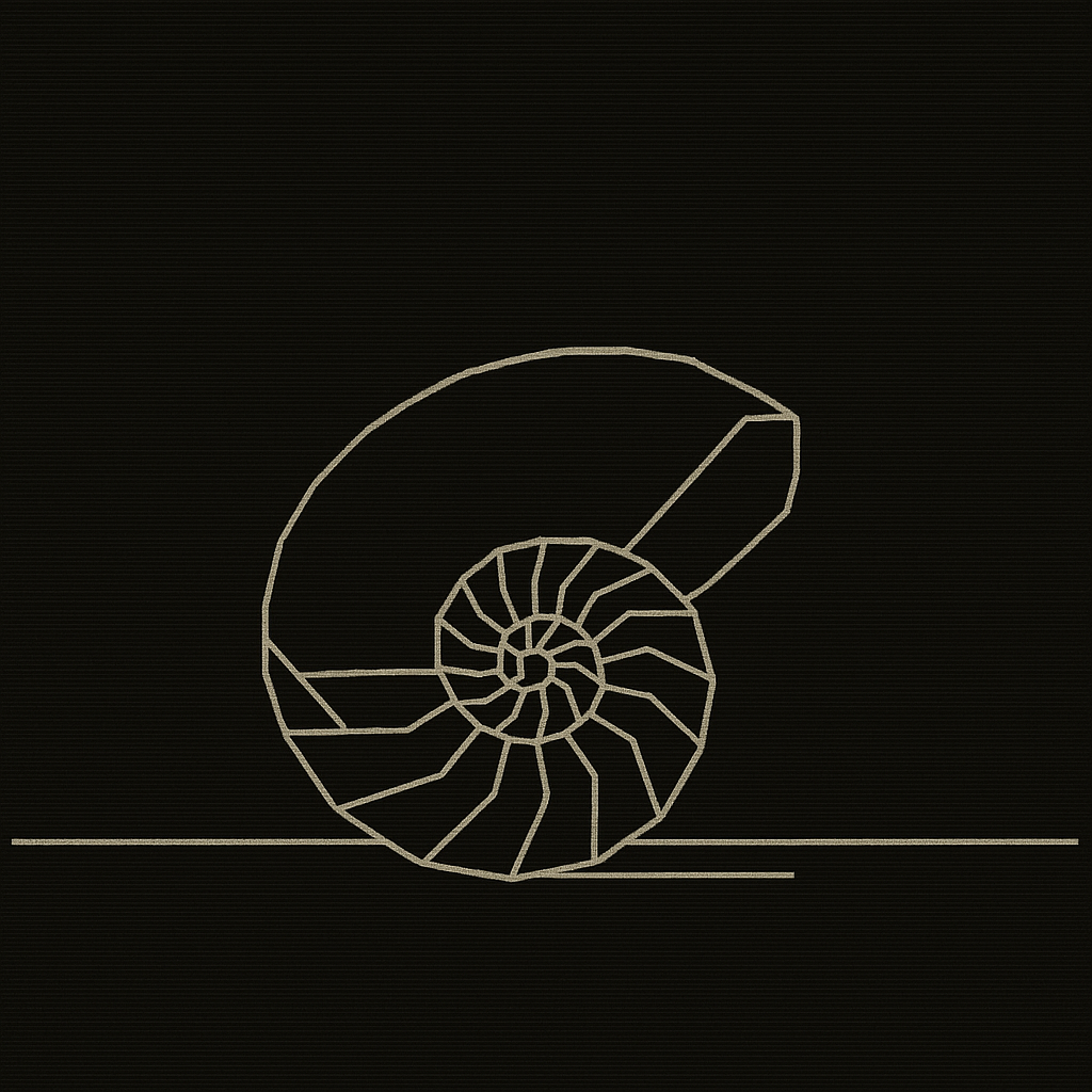
THE MACHINERY OF SPIRAL
A Complete Guide to Rotation Under Radial Change
How the Geometry of Non-Closing Orbits Actually Works
What follows is not metaphor.
It is not a meditation on growth. Not a spiritual symbol. Not a loose analogy between seashells and galaxies dressed in mystical clothing.
It is mechanism.
The actual mathematics of what happens when a system rotates and simultaneously moves toward or away from its center. The physics of trajectories that refuse to close.
A circle closes. A straight line does not curve. Between these two lives the spiral. A path that turns and turns and never returns to where it started.
Most people see spirals everywhere and think it is coincidence. Hurricanes. Galaxies. Sunflower heads. The cochlea of the inner ear. Water draining from a bathtub. The arms of the Milky Way.
It is not coincidence.
It is the generic trajectory of systems with two simultaneous properties: angular motion and radial change. Eliminate either one and the spiral disappears. A system that rotates without radial change traces a circle. A system that moves radially without rotation traces a line. The spiral is what happens when both are present.
This document is about the conditions that produce that combination. Where it appears in nature. What it reveals about the systems generating it. And the constraints that govern when spirals form, when they persist, and when they break.
PART ONE: THE EQUATION
Two Ingredients
Every spiral in every domain reduces to the same structural recipe.
Ingredient one: angular displacement. The system moves around a center. It accumulates angle over time.
Ingredient two: radial change. The distance from the center is not constant. It grows, shrinks, or both.
That is the entire recipe.
When these two ingredients combine, the resulting trajectory is a spiral. The specific relationship between angular rate and radial rate determines which type of spiral appears.
    THE TWO INGREDIENTS

    ┌───────────────────────┐      ┌───────────────────────┐
    │                       │      │                       │
    │   ANGULAR MOTION      │      │   RADIAL CHANGE       │
    │                       │      │                       │
    │   Rotation around     │      │   Distance from       │
    │   a center point      │      │   center increases    │
    │                       │  +   │   or decreases        │
    │   Without this:       │      │                       │
    │   straight line       │      │   Without this:       │
    │                       │      │   circle              │
    └───────────────────────┘      └───────────────────────┘
                   │                          │
                   └────────────┬─────────────┘
                                │
                                ▼
                   ┌───────────────────────┐
                   │                       │
                   │        SPIRAL         │
                   │                       │
                   │   A trajectory that   │
                   │   turns and never     │
                   │   closes              │
                   │                       │
                   └───────────────────────┘
In polar coordinates, a spiral is any curve where the radius r is a non-constant function of the angle θ. That is all. The equation r = f(θ) with f not constant generates a spiral.
The Three Fundamental Types
The relationship between r and θ determines the spiral’s character.
Archimedean spiral. r = a + bθ. The radius grows linearly with angle. Each successive ring is exactly the same distance from the previous one. The groove on a vinyl record. The coil of a clock spring. Equal spacing, constant growth rate.
Logarithmic spiral. r = ae^(bθ). The radius grows exponentially with angle. Each successive ring is a fixed multiple wider than the previous one. The nautilus shell. The hurricane. Proportional spacing, accelerating growth.
Fermat spiral. r = a√θ. The radius grows as the square root of angle. Each successive ring is closer together than the previous one. Decelerating growth, converging density. The arrangement of seeds in a sunflower head.
    THREE SPIRAL TYPES

    ARCHIMEDEAN               LOGARITHMIC              FERMAT
    r = a + bθ                r = ae^(bθ)              r = a√θ

    Ring spacing:             Ring spacing:             Ring spacing:
    CONSTANT                  INCREASING               DECREASING

         ┌───┐                     ┌──┐                    ┌────┐
        /     \                   / ┌─┐\                  /  ┌┐  \
       │ ┌───┐ │                 │/    \│                │  ││││  │
       │ │   │ │                 ││    ││                │  │└┘│  │
       │ └───┘ │                 │\    /│                │  └──┘  │
        \     /                   \ └─┘/                  \      /
         └───┘                     └──┘                    └────┘

    Equal gaps               Gaps widen                Gaps narrow
    between turns            exponentially             toward center
The type of spiral is a fingerprint. It reveals the dynamical law governing the radial change.
Linear growth produces Archimedean. Proportional growth produces logarithmic. Decelerating growth produces Fermat.
Read the spacing between turns and you read the law.
PART TWO: THE SPIRA MIRABILIS
The Logarithmic Spiral and Self-Similarity
In 1692, Jacob Bernoulli published a paper on what he called the spira mirabilis. The marvelous spiral.
What made it marvelous was a single property.
Scale it up or down and it looks the same.
Rotate it and it looks the same.
Take any portion of it and the portion is geometrically similar to the whole.
No other spiral has this property. The Archimedean spiral changes shape at different scales. The Fermat spiral changes shape. Only the logarithmic spiral is self-similar.
The reason is the equiangular property. At every point on a logarithmic spiral, the angle between the tangent line and the radius vector is the same. It does not matter where on the spiral you measure. The angle is constant.
    THE EQUIANGULAR PROPERTY

              tangent
             ╱
            ╱
           ╱  ψ
          ╱────
         •─────────────── radius to center
        (any point
         on spiral)


    ψ = constant everywhere on the curve

    Archimedean:  ψ changes at every point
    Logarithmic:  ψ is the same at every point
    Fermat:       ψ changes at every point


    ψ determines the spiral's tightness:
    ┌──────────────────────────────────────────┐
    │  ψ → 90°    Spiral approaches circle    │
    │  ψ → 0°     Spiral approaches line      │
    │  ψ = 73°    Golden spiral               │
    └──────────────────────────────────────────┘
This constancy has a mathematical consequence. The differential equation generating a logarithmic spiral is dr/dθ = br. The rate of radial change is proportional to the current radius. This is the signature of exponential processes.
Every system that grows proportionally to its current size, while rotating, produces a logarithmic spiral.
Compound interest with rotation. Population growth with rotation. Autocatalytic reaction with rotation.
The logarithmic spiral is the spatial trace of exponential dynamics in a rotating frame.
Why Nature Favors the Logarithmic
The self-similarity of the logarithmic spiral has a consequence that biology exploits.
An organism can grow by adding material at one end without changing its shape. The nautilus adds chamber after chamber, each proportionally larger than the last, and the overall form remains geometrically identical at every stage. No remodeling. No reshaping. Just accretion at the growth edge.
This is the cheapest possible growth strategy. Build more of the same, slightly larger. The blueprint never changes.
D’Arcy Thompson recognized this in 1917. The logarithmic spiral is the form that allows growth without change of shape. Any other growth law would require the organism to continuously restructure its existing form.
A horn. A tusk. A claw. A shell. A ram’s horn. A hawk’s talon. The spiral structures of biology are overwhelmingly logarithmic because logarithmic growth is the only growth that preserves geometry.
PART THREE: THE PHASE PORTRAIT
Complex Eigenvalues
The deepest reason spirals are universal has nothing to do with biology or aesthetics.
It is linear algebra.
Consider any system near an equilibrium point. Two variables interacting. The behavior near equilibrium is governed by a 2x2 matrix. The eigenvalues of that matrix determine the trajectory.
Real eigenvalues produce straight trajectories. Nodes. Direct approach to or departure from equilibrium.
Complex eigenvalues produce spirals.
The imaginary part of the eigenvalue creates the rotation. The real part creates the radial change.
    EIGENVALUE ANATOMY AND TRAJECTORY

    Eigenvalue: λ = α ± βi

    ┌──────────────────────────────────────────────────────┐
    │                                                      │
    │   α (real part)        β (imaginary part)            │
    │   ═══════════          ═══════════════               │
    │                                                      │
    │   Controls radial      Controls angular              │
    │   behavior             behavior                      │
    │                                                      │
    │   α < 0 → decay        β determines                 │
    │   α > 0 → growth       rotation speed               │
    │   α = 0 → neither                                   │
    │                                                      │
    └──────────────────────────────────────────────────────┘
                        │
                        ▼

    α < 0               α = 0               α > 0
    SPIRAL SINK          CENTER              SPIRAL SOURCE

         ╲  ╱                │                   ╱  ╲
          ╲╱             ┌───┴───┐              ╱    ╲
           •             │   •   │             •
          ╱╲             └───┬───┘              ╲    ╱
         ╱  ╲                │                   ╲  ╱

    Spirals inward       Perfect circles     Spirals outward
    (stable)             (marginally         (unstable)
                          stable)
This is why spirals appear in nearly every dynamical system. Complex eigenvalues are not exotic. They are the generic case. Two interacting variables with any rotational component in their coupling will produce complex eigenvalues.
The special case is real eigenvalues. Straight-line approach to equilibrium requires a specific structural condition: the two variables must not create any rotational interaction. This is the exception, not the rule.
Spirals are the default trajectory near equilibrium.
The Spiral Sink
When the real part of the eigenvalue is negative, the system spirals inward. Each orbit is smaller than the last. The trajectory converges to the equilibrium.
This is stable equilibrium with oscillatory approach.
A marble in a bowl of honey. It circles toward the bottom, each revolution tighter. The rotation comes from angular momentum. The decay comes from viscous dissipation.
A damped electrical oscillator. Current spirals down in the phase plane of voltage and current. Each cycle smaller. The resistance is the dissipation. The inductance and capacitance create the rotation.
The spiral sink is the signature of stability with delay. The system returns to equilibrium, but not directly. It overshoots. Corrects. Overshoots again. Each overshoot smaller than the last.
    SPIRAL SINK IN PHASE SPACE

    Variable B
         │
         │        ╲
         │     ╲   ╲
         │      ╲   │
         │       │  │
         │       │  •  ← equilibrium
         │       │ ╱
         │      ╱ ╱
         │     ╱
         │
         └──────────────────────────────────►
                   Variable A

    Trajectory spirals inward.
    Each revolution closer to center.
    System settles to rest.
PART FOUR: THE HOPF BIFURCATION
When Spirals Give Birth to Cycles
The most consequential transition in dynamical systems theory involves a spiral.
Consider a spiral sink. The real part α of the eigenvalue is negative. The system spirals inward. Stable.
Now vary a parameter. Temperature. Concentration. Flow rate. Any control variable.
As the parameter changes, α increases. The spiral weakens. Each revolution decays less. The inward pull softens.
At α = 0, the spiral becomes a center. Perfect circles. No growth, no decay. Marginally stable.
Push the parameter further. α becomes positive. The spiral reverses. Now it spirals outward. Each revolution larger. The equilibrium has become unstable.
But something must contain the growth. No physical system expands forever. Nonlinear terms kick in. They arrest the expansion. The outward spiral locks onto a closed orbit.
A limit cycle is born.
This is the Hopf bifurcation.
    THE HOPF BIFURCATION

    BEFORE (α < 0)          AT (α = 0)           AFTER (α > 0)
    ────────────────         ────────────         ────────────────

         ╲  ╱                  ┌─────┐              ╱  ╲
          ╲╱                  │     │             ╱ ┌──┐ ╲
           •                  │  •  │            │ │  │ │
          ╱╲                  │     │             ╲ └──┘ ╱
         ╱  ╲                  └─────┘              ╲  ╱

    Spiral sink             Center               Limit cycle
    All trajectories        Closed orbits         Stable periodic
    decay to point                                orbit attracts
                                                  all trajectories


    PARAMETER ──────────────────────────────────────────►
                        ▲
                        │
                   Critical point:
                   spiral → cycle
The heartbeat originates this way. Cardiac pacemaker cells sit near a Hopf bifurcation. Below threshold, they spiral to a resting potential. Above threshold, they lock onto a limit cycle. The oscillation is born from the spiral.
The Belousov-Zhabotinsky chemical oscillation works the same way. Below critical concentration, the reaction spirals to a steady state. Above it, oscillation appears.
The transition from silence to oscillation, from rest to rhythm, from stillness to pulse. In system after system, that transition passes through a spiral.
PART FIVE: SPIRAL WAVES
Rotation in Extended Media
Spirals do not only appear as trajectories of point systems. They appear as spatial patterns in extended media.
An excitable medium is a material that can be triggered. Push it past a threshold and it fires. Then it enters a refractory period where it cannot fire again. After recovery, it is ready.
Neurons. Cardiac tissue. The BZ chemical reaction in a dish. Slime mold colonies.
When such a medium is triggered at a single point, a circular wave expands outward. Like a stone dropped in a pond.
But when the trigger meets a broken wavefront, something different happens. The wavefront curls. The broken end becomes a pivot. The wave rotates around that point.
A spiral wave is born.
    SPIRAL WAVE FORMATION

    1. INTACT WAVE              2. BROKEN WAVEFRONT
       (circular)                  (one end free)

        ┌────────┐                 ┌──────
        │        │                 │
        │   •    │                 │   •
        │        │                 │
        └────────┘                 └──────
                                        ▲
                                        │
                                   free end curls


    3. SPIRAL FORMS              4. STEADY ROTATION

            ╱                         ╱╲
           ╱                         ╱  ╲
          •                         •    │
           ╲                         ╲  ╱
            ╲                         ╲╱

       Free end pivots            Continuous rotation
       around the tip             around the spiral core
The tip of the spiral is the organizing center. Everything rotates around it. The spiral wave is a self-sustaining rotor in the medium.
Arthur Winfree recognized this in the 1970s. He showed that spiral waves are topological objects. They carry a topological charge. They cannot be created or destroyed singly. They form in pairs of opposite rotation, and they can only be annihilated in pairs.
The Cardiac Rotor
The most consequential spiral wave in nature forms in the heart.
Normal cardiac rhythm is a planar wave. The electrical signal propagates smoothly from the sinoatrial node through the atria, through the conduction system, through the ventricles. Coordinated contraction.
When this wave encounters damaged tissue, a scar, an ischemic region, the wavefront can break. One end becomes free. It curls. A spiral wave forms.
The spiral wave is a reentrant circuit. The electrical signal chases its own tail, rotating around the spiral core at a rate faster than the normal heartbeat.
This is ventricular tachycardia.
If the spiral becomes unstable and breaks into multiple spirals, the result is ventricular fibrillation. Disordered electrical activity. No coordinated contraction. Without intervention, death in minutes.
A defibrillator works by overwhelming the spiral. The massive electrical shock resets every cell simultaneously, destroying all spiral waves and allowing the normal conduction pathway to reassert itself.
The spiral is the mechanism of sudden cardiac death. Understanding that mechanism is what makes defibrillation rational rather than empirical.
PART SIX: THE GALAXY
The Winding Problem
Spiral galaxies present a puzzle.
Stars near the center orbit faster than stars at the edge. Differential rotation. The inner stars complete an orbit in tens of millions of years. The outer stars take hundreds of millions.
If the spiral arms were material structures, made of the same stars at each moment, differential rotation would wind them up. Within a few galactic rotations, the arms would wrap tighter and tighter until they disappeared into a featureless disk.
But spiral galaxies persist for billions of years. Hundreds of rotation periods. The arms should have wound up long ago.
They haven’t.
    THE WINDING PROBLEM

    IF ARMS WERE MATERIAL:

    Time 0              Time 1              Time 2
    ┌─────────┐         ┌─────────┐         ┌─────────┐
    │  ╱      │         │ ╱╱      │         │╱╱╱╱     │
    │ ╱   •   │         │╱╱   •   │         │╱╱╱  •   │
    │╱        │         │╱        │         │╱        │
    └─────────┘         └─────────┘         └─────────┘

    Arms wrap tighter and tighter.
    After ~500 million years: featureless disk.

    OBSERVED REALITY:
    Spiral arms persist for billions of years.
    Something else is happening.
Density Waves
In 1964, C.C. Lin and Frank Shu proposed the solution.
The spiral arms are not material. They are density waves. Compression patterns moving through the disk of stars and gas.
Think of a traffic jam on a circular highway. Cars slow down when they enter the congested zone. They pile up. The density increases. Then they accelerate out the other side. The cars pass through the jam. But the jam persists.
The jam is not made of the same cars at each moment. It is a pattern, a region of higher density, through which cars flow.
Spiral arms work the same way.
Stars orbit the galactic center on their own trajectories. When they enter the density wave, they slow down. They pile up. The density increases. Gas is compressed. New stars form. The bright young stars illuminate the arm.
Then the stars pass through and continue their orbit. But the density wave remains.
The pattern rotates at a fixed angular speed, the pattern speed, which is different from the orbital speed of any individual star. Stars at different radii pass through the pattern at different rates. But the pattern itself is stable.
    DENSITY WAVE MECHANISM

    ┌──────────────────────────────────────────────────┐
    │                                                  │
    │   STARS move at orbital velocity (varies         │
    │   with radius, faster near center)               │
    │                                                  │
    │   PATTERN moves at pattern speed (constant,      │
    │   independent of radius)                         │
    │                                                  │
    │   Stars pass THROUGH the pattern.                │
    │   The pattern persists.                          │
    │                                                  │
    └──────────────────────────────────────────────────┘

    ┌────────────────────┐      ┌────────────────────┐
    │                    │      │                    │
    │   TRAFFIC JAM      │      │   SPIRAL ARM       │
    │                    │      │                    │
    │   Cars flow        │      │   Stars flow       │
    │   through it       │      │   through it       │
    │                    │      │                    │
    │   Jam stays        │      │   Arm stays        │
    │                    │      │                    │
    └────────────────────┘      └────────────────────┘
The spiral is not a thing. It is a process. A standing wave in a rotating medium. The form persists while the material passes through.
PART SEVEN: THE GROWTH SPIRAL
Phyllotaxis
The arrangement of leaves, seeds, and petals on plants follows spiral patterns with eerie mathematical precision.
Count the spirals on a sunflower head. You find 34 spirals going one way, 55 going the other. Or 55 and 89. Or 89 and 144.
These are consecutive Fibonacci numbers.
This is not numerology. It is geometry.
In 1992, Stéphane Douady and Yves Couder demonstrated the mechanism with an experiment using magnetized ferrofluid droplets. Successive drops fell onto a dish. Each drop repelled every other drop. The drops were carried outward by the field.
The drops spontaneously arranged into Fibonacci spirals.
No biology. No genetics. No programming. Pure physics. Repulsion plus radial growth.
The mechanism is this. Each new primordium (bud, seed, leaf) forms at the growing tip. It is pushed outward by subsequent growth. It repels nearby primordia. The system seeks to place each new element as far as possible from existing ones.
The angle that maximizes packing is the golden angle: 137.5 degrees.
    THE GOLDEN ANGLE AND FIBONACCI SPIRALS

    Why 137.5°?

    360° × (1 - 1/φ) = 360° × (1 - 0.618...) = 137.507...°

    where φ = (1 + √5)/2 = the golden ratio


    ┌──────────────────────────────────────────────────┐
    │                                                  │
    │   Each new element placed 137.5° from the last   │
    │                                                  │
    │   This angle is the MOST IRRATIONAL rotation.    │
    │   It avoids resonance with any rational           │
    │   fraction of a full turn.                       │
    │                                                  │
    │   Result: no two elements ever line up            │
    │   radially. Maximum packing efficiency.          │
    │                                                  │
    │   The Fibonacci spiral counts are a               │
    │   consequence of this angle, not a cause.        │
    │                                                  │
    └──────────────────────────────────────────────────┘
The golden angle is the most irrational number in a precise sense. Its continued fraction representation is [1; 1, 1, 1, …]. It converges to its rational approximations more slowly than any other irrational number. This means elements placed at golden-angle intervals are maximally resistant to forming radial alignments.
The Fibonacci numbers appear because they are the convergents of this continued fraction. They are the best rational approximations to the golden ratio. When you count spirals, you count these convergents.
The plant does not know the Fibonacci sequence. It does not compute the golden ratio. It grows with repulsion and radial expansion. The mathematics is emergent.
The Cochlea
The spiral of the inner ear is not decorative.
The cochlea coils approximately 2.5 turns. Along its length, the basilar membrane varies in width and stiffness. Narrow and stiff at the base. Wide and flexible at the apex.
This gradient creates a tonotopic map. High frequencies activate the base. Low frequencies activate the apex. The mapping is logarithmic. Each octave of frequency occupies approximately equal physical distance along the membrane.
The Greenwood function describes this: f = A(10^(ax) - k), where x is the position along the basilar membrane and f is the characteristic frequency.
The spiral geometry is not incidental. It allows the cochlea to pack a long membrane into a compact space. The human basilar membrane is approximately 35 millimeters long. Uncoiled, it would not fit in the temporal bone. The spiral is a packing solution.
But the spiral shape may also contribute to the frequency response itself. The curvature produces a radial pressure gradient that enhances low-frequency sensitivity at the apex, exactly where the membrane is widest and most flexible.
Form serves function. The spiral is simultaneously structure, compression, and amplification.
PART EIGHT: THE STRANGE ATTRACTOR
When Spirals Go Chaotic
In 1976, Otto Rössler constructed the simplest possible system that produces chaos. Three differential equations. One nonlinear term.
The Rössler attractor is built from a spiral.
Most of the time, the trajectory spirals outward in a plane. Each revolution slightly larger than the last. A spiral source.
But there is a boundary. When the trajectory gets too far from center, it is kicked upward in the third dimension. Then it falls back to the plane. And begins spiraling again.
The spiral stretches. The reinjection folds. Stretch and fold, stretch and fold. This is the recipe for chaos.
    THE RÖSSLER ATTRACTOR

    TOP VIEW (x-y plane):        SIDE VIEW (x-z plane):

         ╱──────╲                         ╱╲
        ╱ ╱────╲ ╲                       ╱  │
       │ ╱      ╲ │                     ╱   │
       ││   •    ││                    ╱    │  ← reinjection
       │ ╲      ╱ │               ────╱     │     (fold)
        ╲ ╲────╱ ╱                          │
         ╲──────╱                    ────────┘
                                     spiraling
    Outward spiral                   (stretch)
    in the plane


    THE MECHANISM OF CHAOS:

    ┌──────────┐     ┌──────────┐     ┌──────────┐
    │          │     │          │     │          │
    │  SPIRAL  │ ──► │  REACH   │ ──► │  FOLD    │
    │  OUTWARD │     │  BOUNDARY│     │  BACK    │
    │          │     │          │     │          │
    └──────────┘     └──────────┘     └──────────┘
         ▲                                 │
         │                                 │
         └─────────────────────────────────┘
               Reinjection at different
               phase each time = chaos
The key is that the reinjection does not return the trajectory to the same point. Each time the spiral reaches the boundary and folds back, it arrives at a slightly different phase. The spiral begins again from a different position. After many iterations, the trajectory never repeats. It is aperiodic. Deterministic but unpredictable.
The Rössler attractor reveals something fundamental. Chaos is not randomness. It is a spiral that never quite closes. A trajectory that almost repeats, spiraling through nearly the same region of phase space again and again, but always displaced by the folding.
Chaos is the spiral’s failure to return.
PART NINE: THE PARTICLE
Cyclotron Motion
A charged particle in a uniform magnetic field traces a circle. The magnetic force is perpendicular to both the velocity and the field. It bends the trajectory without changing the speed.
But add any energy loss and the circle becomes a spiral.
The particle radiates as it accelerates around the curve. Cyclotron radiation at low speeds. Synchrotron radiation at relativistic speeds. Each revolution, the particle loses energy. Its speed decreases. The radius of curvature shrinks.
The trajectory spirals inward.
    CHARGED PARTICLE SPIRAL

    Magnetic field B
    (pointing out of page)
    ⊙  ⊙  ⊙  ⊙  ⊙

         ╲
          ╲
           ╲
            ╲ ╱──╲
             ╱ ╱─╲ ╲
            │ │ • │ │
             ╲ ╲─╱ ╱
              ╲──╱
               trajectory spirals
               inward as particle
               radiates energy


    No radiation → circle (constant radius)
    With radiation → spiral (shrinking radius)

    Energy loss per revolution:
    ΔE ∝ q²B²v² / (m²c³)

    The spiral is the trajectory of
    dissipation in a rotating system.
This is the same structure as the spiral sink in the phase portrait. The magnetic field provides the rotation. The radiation provides the dissipation. Together they produce a spiral.
The synchrotron is built on this principle. Charged particles spiral through magnetic fields, and the radiation they emit becomes the light source. X-ray crystallography. Protein structure determination. Materials science. The spiral of a decaying particle orbit became one of the most productive tools in modern science.
PART TEN: THE CONSTRAINTS
Why Spirals Are Generic
The universality of spirals is not mysterious. It follows from a mathematical fact.
In two-dimensional dynamical systems, the behavior near an equilibrium depends on the eigenvalues of the linearized system. For a 2x2 real matrix, the eigenvalues are either both real or a complex conjugate pair.
Real eigenvalues require the discriminant of the characteristic polynomial to be non-negative. This is a codimension-zero condition. It defines a region in parameter space.
Complex eigenvalues require the discriminant to be negative. This is also a codimension-zero condition. It defines the complementary region.
Neither condition is special. Both occupy open sets in parameter space. But complex eigenvalues are “typical” in the sense that a randomly chosen 2x2 matrix is more likely to have complex eigenvalues than repeated real eigenvalues.
    EIGENVALUE PARAMETER SPACE

    Parameter B
         │
         │   ┌──────────────────────────────────┐
         │   │                                  │
         │   │      COMPLEX EIGENVALUES         │
         │   │      (spiral trajectories)       │
         │   │                                  │
         │   │          ┌────────────────┐       │
         │   │          │ REAL EIGENVALUES│      │
         │   │          │ (node/saddle)  │       │
         │   │          └────────────────┘       │
         │   │                                  │
         │   │                                  │
         │   └──────────────────────────────────┘
         │
         └──────────────────────────────────────────►
                   Parameter A

    Both regions have nonzero measure.
    But coupling between variables
    generically produces complex eigenvalues.

    The more two variables interact,
    the more likely the spiral.
Any system with two interacting components that involve any rotational coupling will generically produce spirals. Predator-prey interactions, electrical oscillators, chemical reactions with competing pathways, fluid instabilities with rotation.
The spiral is the default, not the exception.
The Relationship to the Exponential
The logarithmic spiral has a deep connection to the exponential function.
In the complex plane, the exponential e^(α+iβ)t traces a spiral when α is nonzero. The imaginary part βt generates rotation. The real part αt generates radial growth or decay.
The spiral IS the exponential function visualized in two dimensions.
This is why spirals appear wherever exponential processes interact with periodic processes. Growth with oscillation. Decay with rotation. Inflation with cycling. Dissipation with orbiting.
    SPIRAL AS COMPLEX EXPONENTIAL

    e^(α+iβ)t = e^(αt) × [cos(βt) + i sin(βt)]

    ┌──────────────────────────────────────────────────┐
    │                                                  │
    │   e^(αt)           Growth/decay envelope         │
    │                    (radial component)             │
    │                                                  │
    │   cos(βt)          Oscillation in x              │
    │   sin(βt)          Oscillation in y              │
    │                    (angular component)            │
    │                                                  │
    │   Together:        SPIRAL                        │
    │                                                  │
    │   α < 0  →  decaying spiral  (sink)              │
    │   α = 0  →  circle           (center)            │
    │   α > 0  →  growing spiral   (source)            │
    │                                                  │
    └──────────────────────────────────────────────────┘
The exponential is the mother function. In one dimension it produces growth or decay. In two dimensions it produces spirals. In all dimensions it describes processes where the rate of change is proportional to the current state.
When Spirals Break
Spirals are robust but not indestructible. Several conditions destroy them.
Loss of rotation. If the coupling between variables becomes purely cooperative or purely competitive, the imaginary part of the eigenvalue vanishes. The spiral collapses to a node. Direct approach or departure, no winding.
Bifurcation. As parameters change, the eigenvalues can shift. Complex to real. Spiral to node. Or complex to larger complex. Spiral to chaos. The Hopf bifurcation creates limit cycles. Other bifurcations can destroy spirals entirely.
Symmetry constraints. In systems with exact symmetry, eigenvalues can be forced to be real. Perfect symmetry prohibits rotation. The spiral requires some asymmetry in the interaction.
Dimension reduction. If one variable becomes much faster than the other, it equilibrates instantly. The system effectively becomes one-dimensional. One-dimensional systems cannot spiral. They can only grow or decay.
The spiral requires at least two dimensions, some rotational coupling, and eigenvalues with nonzero imaginary parts. Remove any of these and the spiral vanishes.
PART ELEVEN: THE COMPLETE PICTURE
The Unified View
Everything connects through the two ingredients.
    THE SPIRAL ACROSS DOMAINS

    ┌──────────────────────────────────────────────────────────┐
    │                    THE SPIRAL IS                          │
    │                                                          │
    │        ROTATION  +  RADIAL CHANGE                        │
    │                                                          │
    │   Wherever these two coexist, a spiral appears.          │
    └──────────────────────────────────────────────────────────┘
                              │
            ┌─────────────────┼─────────────────┐
            │                 │                 │
            ▼                 ▼                 ▼
    ┌──────────────┐  ┌──────────────┐  ┌──────────────┐
    │  DYNAMICAL   │  │  PHYSICAL    │  │  BIOLOGICAL  │
    │  SYSTEMS     │  │  SYSTEMS     │  │  SYSTEMS     │
    │              │  │              │  │              │
    │  Phase       │  │  Galaxies    │  │  Shells      │
    │  portraits   │  │  Particles   │  │  Phyllotaxis │
    │  Attractors  │  │  Hurricanes  │  │  Cochlea     │
    │  Bifurcation │  │  Vortices    │  │  DNA helix   │
    └──────────────┘  └──────────────┘  └──────────────┘
            │                 │                 │
            └─────────────────┼─────────────────┘
                              │
                              ▼
    ┌──────────────────────────────────────────────────────────┐
    │                                                          │
    │   The spiral is the complex exponential made visible.    │
    │   Growth or decay, combined with periodicity.            │
    │   The most natural trajectory in systems with            │
    │   two interacting variables and rotational coupling.     │
    │                                                          │
    └──────────────────────────────────────────────────────────┘
The spiral sink is how stable systems settle. Not directly. Through oscillatory decay. The approach to rest is winding.
The spiral source is how instabilities grow. Not directly. Through oscillatory expansion. The departure from rest is winding.
The Hopf bifurcation is how spirals birth cycles. The transition from rest to rhythm passes through the spiral.
The spiral wave is how extended media sustain rotation. Cardiac arrhythmia. Chemical oscillation. Biological signaling.
The density wave is how galaxies maintain structure. The spiral pattern persists while stars flow through it. Form without material permanence.
The logarithmic spiral is how organisms grow. The only geometry that preserves shape under proportional growth.
The strange attractor is how spirals generate chaos. Almost closing, never quite closing. Deterministic but unpredictable.
The charged particle is how spirals encode dissipation. Every lost quantum of energy tightens the curve.
The Observation
The spiral is not a shape. It is a process.
It is what happens when rotation and radial change coexist. And they coexist almost everywhere. Because almost every system with two interacting components has some rotational coupling in its dynamics. Because complex eigenvalues are generic. Because the exponential function, when given an imaginary component, spirals.
The circle is the special case. Pure rotation. No radial change. No growth. No decay. The circle requires perfect conservation. No friction, no dissipation, no input, no output.
The real world has friction. Has dissipation. Has growth and decay.
The real world spirals.
Not as metaphor. As mathematics.
The equations do not choose to spiral any more than water chooses to flow downhill. The spiral is the geometric consequence of the most common dynamical conditions in nature.
That is the machinery. Not what the spiral symbolizes. What it is.
Rotation plus radial change. Two ingredients. One geometry. Everywhere.
Citations
Mathematics
Bernoulli, J. (1692). “Spira mirabilis.” Acta Eruditorum. (The original description of the logarithmic spiral’s self-similarity and equiangular property.)
Thompson, D.W. (1917). On Growth and Form. Cambridge University Press. (Foundational work connecting logarithmic spirals to biological growth.)
Strogatz, S.H. (2015). Nonlinear Dynamics and Chaos: With Applications to Physics, Biology, Chemistry, and Engineering. 2nd ed. Westview Press. (Standard reference for phase portraits, eigenvalue classification, Hopf bifurcation, limit cycles.)
Dynamical Systems
Rössler, O.E. (1976). “An equation for continuous chaos.” Physics Letters A, 57(5):397-398. (The simplest chaotic attractor with spiral structure.)
Marsden, J.E. & McCracken, M. (1976). The Hopf Bifurcation and Its Applications. Springer. (Mathematical foundations of the spiral-to-limit-cycle transition.)
Guckenheimer, J. & Holmes, P. (1983). Nonlinear Oscillations, Dynamical Systems, and Bifurcations of Vector Fields. Springer. (Classification of equilibria, spiral sinks/sources, complex eigenvalues.)
Spiral Waves
Winfree, A.T. (1972). “Spiral waves of chemical activity.” Science, 175(4022):634-636. (Discovery of spiral waves in the BZ reaction.)
Davidenko, J.M., et al. (1992). “Stationary and drifting spiral waves of excitation in isolated cardiac muscle.” Nature, 355:349-351. (Spiral wave reentry in cardiac tissue.)
Jalife, J. (2000). “Ventricular fibrillation: mechanisms of initiation and maintenance.” Annual Review of Physiology, 62:25-50.
Astrophysics
Lin, C.C. & Shu, F.H. (1964). “On the spiral structure of disk galaxies.” The Astrophysical Journal, 140:646-655. (The density wave theory of spiral arms.)
Bertin, G. & Lin, C.C. (1996). Spiral Structure in Galaxies: A Density Wave Theory. MIT Press.
Biology
Douady, S. & Couder, Y. (1992). “Phyllotaxis as a physical self-organized growth process.” Physical Review Letters, 68(13):2098-2101. (Experimental demonstration that Fibonacci spirals arise from repulsion plus radial growth.)
Jean, R.V. (1994). Phyllotaxis: A Systemic Study in Plant Morphogenesis. Cambridge University Press.
Greenwood, D.D. (1990). “A cochlear frequency-position function for several species: 29 years later.” Journal of the Acoustical Society of America, 87(6):2592-2605. (The logarithmic frequency map of the cochlea.)
Physics
Jackson, J.D. (1998). Classical Electrodynamics. 3rd ed. Wiley. (Charged particle motion in magnetic fields, cyclotron and synchrotron radiation.)
Rybicki, G.B. & Lightman, A.P. (1979). Radiative Processes in Astrophysics. Wiley. (Synchrotron radiation and spiral particle trajectories.)
Related Machineries
- THE MACHINERY OF CYCLES. Cycles are closed orbits. Spirals are orbits that fail to close. The spiral is the generic trajectory near an equilibrium that, under specific conditions, can tighten into a cycle via the Hopf bifurcation.
- THE MACHINERY OF ATTRACTOR. The spiral sink is a point attractor approached through winding trajectories. Spiral structure determines how systems converge to their attractors.
- THE MACHINERY OF BIFURCATION. The Hopf bifurcation is the canonical spiral-to-cycle transition, where the spiral’s radial component crosses zero and a limit cycle is born.
- THE MACHINERY OF OSCILLATION. Damped oscillations are spirals in phase space. The relationship between oscillation and spiral is one of projection: the oscillation is the time-series view, the spiral is the phase-space view.