THE MACHINERY OF SYNCHRONIZATION
A Complete Guide to Coupled Oscillators
How Independent Systems Lock Into Collective Order
What follows is not advice.
It is not a framework for alignment, teamwork, or getting people on the same page. Not a metaphor borrowed from physics to dress up a management concept.
It is mechanism.
The actual mathematics of how independent oscillating systems abandon their own rhythms and fall into collective phase. The physics of how thousands of fireflies flash in unison without a conductor. The architecture of how your heart cells beat as one without a central clock telling them when to fire.
Synchronization is one of the most pervasive phenomena in nature. It operates in pendulums, neurons, power grids, lasers, chemical reactions, and cardiac tissue. It emerges from a single structural principle repeated at every scale.
This document is that principle.
Nothing more.
What you do with it is your business.
PART ONE: THE SYMPATHY OF CLOCKS
The First Observation
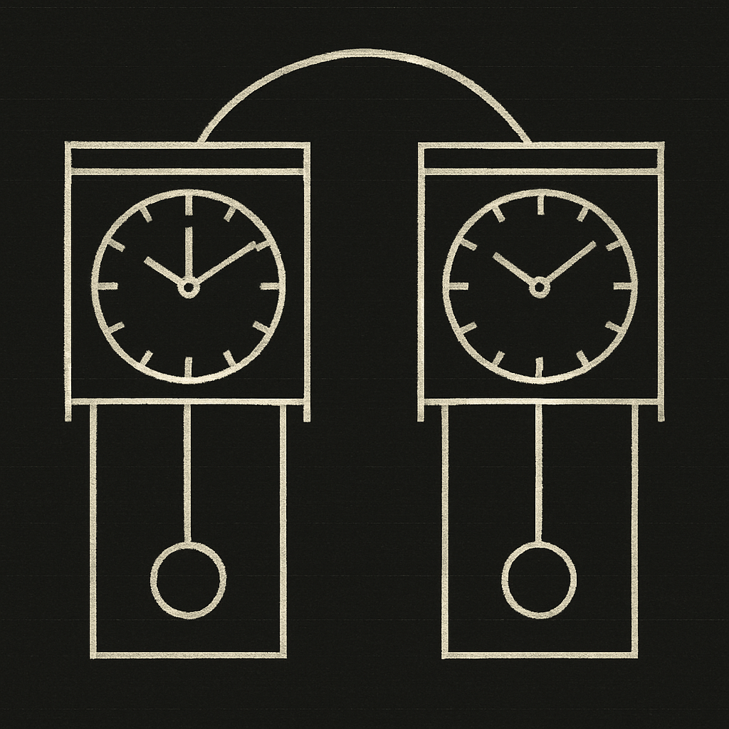
In February 1665, Christiaan Huygens lay ill in his room in The Hague.
Two pendulum clocks hung on the same wooden beam above his bed. He had nothing to do but watch them.
And he noticed something strange.
The two pendulums were swinging in perfect anti-phase. One swung left exactly as the other swung right. Precisely. Continuously. Without anyone setting them that way.
He disturbed them. Stopped one. Started it at a different point in its cycle.
Within thirty minutes, they returned to anti-phase.
Every time.
He called it “une sympathie remarquable.” A remarkable sympathy.
He had discovered synchronization. The first person in recorded history to see it, name it, and attempt to explain it.
What Was Actually Happening
The clocks were not communicating through the air.
They were communicating through the beam.
Each pendulum exerts a tiny lateral force on the mounting structure. The beam flexes. Imperceptibly. That flex transmits force to the other pendulum. The other pendulum responds.
Two oscillators. One coupling medium. Mutual influence.
Anti-phase was the stable state because when the pendulums swing in opposite directions, their forces on the beam cancel. The beam barely moves. Energy stays in the pendulums rather than leaking into the mounting structure.
The system found its own minimum. Not because anyone designed it to. Because the physics demanded it.
    HUYGENS' CLOCKS

    ┌──────────────────────────────────────────────────────┐
    │                  WOODEN BEAM                         │
    │  ════════════════════════════════════════════════     │
    │         │                         │                  │
    │         │                         │                  │
    │        ╱                           ╲                 │
    │       ╱  Clock A                    ╲  Clock B       │
    │      ◄── swings left      swings right ──►           │
    │                                                      │
    │  Forces on beam CANCEL in anti-phase                 │
    │  Beam stays still → energy preserved                 │
    │  Anti-phase is the stable attractor                  │
    └──────────────────────────────────────────────────────┘
This is the template for everything that follows.
Independent oscillators. A coupling channel. Phase adjustment through mutual influence. Convergence to a collective state.
The details change. The structure does not.
PART TWO: THE COUPLING EQUATION
Kuramoto’s Breakthrough
In 1975, Yoshiki Kuramoto wrote down the equation that unified the entire field.
He asked the simplest possible question. Take N oscillators. Each has its own natural frequency. Connect them all to all. What happens?
The equation for each oscillator’s phase:
d(theta_j)/dt = omega_j + (K/N) * sum of sin(theta_k - theta_j)
Three terms. That is all.
The first term is the natural frequency. Each oscillator wants to run at its own speed.
The second term is the coupling. Each oscillator feels a pull toward every other oscillator, proportional to the sine of their phase difference.
K is the coupling strength. One number that controls the entire system.
The Order Parameter
Kuramoto defined a single number that measures how synchronized the population is.
r = magnitude of (1/N) * sum of e^(i * theta_j)
When r = 0, the oscillators are scattered uniformly around the circle. Complete incoherence. No collective rhythm.
When r = 1, every oscillator is at the same phase. Perfect synchrony. One unified pulse.
Between 0 and 1, partial synchronization. Some oscillators locked. Others drifting.
    THE ORDER PARAMETER

    r = 0                    r ≈ 0.5                  r = 1
    INCOHERENT               PARTIAL                  FULL SYNC

    ┌──────────────┐    ┌──────────────┐    ┌──────────────┐
    │   ·  ·       │    │     ·  ·     │    │              │
    │  ·      ·    │    │   ·      ·   │    │              │
    │ ·   ○    ·   │    │  ·   ○       │    │  ·····○      │
    │  ·      ·    │    │       ·  ·   │    │              │
    │   ·  ·       │    │      ·       │    │              │
    └──────────────┘    └──────────────┘    └──────────────┘

    Phases scattered       Cluster forming      All phases aligned
    No collective          Some locked,         Single unified
    rhythm                 some drifting        oscillation
This single number captures the entire macroscopic state of a population of oscillators.
It is the pulse of the collective.
The Critical Threshold
Here is the result that changed everything.
There exists a critical coupling strength K_c. Below it, nothing happens. The oscillators each run at their own frequency. The coupling is too weak to overcome the frequency differences. The system stays incoherent.
At K_c, something breaks. A nucleus of oscillators near the center of the frequency distribution locks together. The order parameter jumps from zero. Synchronization appears.
K_c = 2 / (pi * g(0))
Where g(0) is the height of the frequency distribution at its center. The more concentrated the natural frequencies, the lower the threshold. The more dispersed, the higher.
This is a phase transition. The same mathematics that governs ice becoming water. A qualitative change in the macroscopic state triggered by a quantitative change in a single parameter.
    THE SYNCHRONIZATION PHASE TRANSITION

    Order
    Parameter
    r
         │
    1.0  │                              ─────────────
         │                           ╱
         │                         ╱
         │                       ╱
    0.5  │                     ╱
         │                   ╱
         │                 ╱
         │               ╱
    0.0  │──────────────╱
         │
         └──────────────┬──────────────────────────────► K
                        │
                       K_c
                   (critical coupling)

    Below K_c: incoherence persists regardless of N
    Above K_c: order parameter grows as sqrt(K - K_c)
    Same critical exponent as mean-field magnetization
Below the threshold, the coupling is noise. Each oscillator drifts past the others, pulled briefly but never caught.
Above the threshold, the coupling wins. First a few oscillators lock. Then more are recruited. The synchronized cluster grows, its collective signal strengthening, pulling in oscillators that were previously too fast or too slow.
The rich get richer. The locked group’s signal grows. Weaker oscillators capitulate.
This is not metaphor. This is the mathematics. The same differential equations produce the same dynamics whether the oscillators are neurons, fireflies, or generators on a power grid.
PART THREE: THE MEDIUM
What Carries the Coupling
Huygens’ clocks coupled through a wooden beam.
Metronomes on a shared platform couple through lateral forces on the surface. Pantaleone demonstrated in 2002 that this maps exactly onto the Kuramoto model. In-phase synchronization dominates because it maximizes momentum transfer through the platform.
Cardiac pacemaker cells couple through gap junctions. Direct electrical connections between adjacent cells. Current flows from one cell into the next, pulling their voltage trajectories together.
Power grid generators couple through transmission lines. Reactive power flows between generators that are out of phase, applying torques that pull them back toward synchrony.
Neurons couple through synapses. Chemical or electrical. The signal arrives, shifts the membrane potential, advances or retards the next spike.
    COUPLING MEDIA ACROSS DOMAINS

    ┌──────────────────┐     ┌──────────────────┐
    │   OSCILLATORS    │     │   COUPLING        │
    │                  │     │   MEDIUM           │
    ├──────────────────┤     ├──────────────────┤
    │  Pendulum clocks │ ──► │  Wooden beam      │
    │  Metronomes      │ ──► │  Shared platform  │
    │  Heart cells     │ ──► │  Gap junctions    │
    │  Power generators│ ──► │  Transmission     │
    │                  │     │  lines            │
    │  Neurons         │ ──► │  Synapses         │
    │  Fireflies       │ ──► │  Light pulses     │
    │  Laser arrays    │ ──► │  Optical field    │
    │  Josephson       │ ──► │  Microwave        │
    │  junctions       │     │  radiation        │
    └──────────────────┘     └──────────────────┘
The medium determines everything.
It determines which modes of synchronization are accessible. Huygens’ beam favored anti-phase. A freely sliding platform favors in-phase. Gap junctions favor in-phase. Inhibitory synapses favor anti-phase.
It determines the coupling strength. A rigid beam transmits more force than a flexible one. Dense gap junctions couple more strongly than sparse ones.
It determines the topology. Not all oscillators need to connect to all others. The geometry of connections shapes what synchronization patterns are possible.
The oscillators provide the rhythm. The medium provides the conversation.
PART FOUR: THE PULSE-COUPLED WORLD
Fireflies
Thousands of Pteroptyx fireflies in Southeast Asian mangroves flash in perfect unison.
No conductor. No leader. No central clock.
Each firefly is an integrate-and-fire oscillator. An internal state variable rises toward a threshold. When it reaches threshold, the firefly fires a flash and resets. The cycle begins again.
When a firefly sees a flash from a neighbor, it advances its internal state by a fixed amount. Its own flash comes sooner.
That is the entire mechanism. Receive a pulse. Jump forward. Reset.
In 1990, Mirollo and Strogatz proved the theorem. For N identical integrate-and-fire oscillators with all-to-all excitatory pulse coupling, synchronization occurs for almost all initial conditions.
Almost all. Not all. There exist measure-zero sets of initial conditions that never synchronize. But any infinitesimal perturbation breaks you out of them. In practice, they do not exist.
    PULSE-COUPLED SYNCHRONIZATION

    EARLY STATE:
    ┌──────────────────────────────────────────────────────┐
    │  Firefly A:   ▓▓▓▓▓▓▓▓▓░░░░░│FLASH│ reset          │
    │  Firefly B:   ▓▓▓▓░░░░░░░░░░│     │                 │
    │  Firefly C:   ▓▓▓▓▓▓▓▓▓▓▓░░│     │                 │
    │  Firefly D:   ▓░░░░░░░░░░░░░│     │                 │
    │                                                      │
    │  Phases scattered. Flashes uncorrelated.             │
    └──────────────────────────────────────────────────────┘
                              │
                              │  Each flash advances
                              │  neighbors toward threshold
                              ▼
    ┌──────────────────────────────────────────────────────┐
    │  Firefly A:   ▓▓▓▓▓▓▓▓▓▓▓▓▓│FLASH│ reset            │
    │  Firefly B:   ▓▓▓▓▓▓▓▓▓▓▓▓▓│FLASH│ reset            │
    │  Firefly C:   ▓▓▓▓▓▓▓▓▓▓▓▓▓│FLASH│ reset            │
    │  Firefly D:   ▓▓▓▓▓▓▓▓▓▓▓▓▓│FLASH│ reset            │
    │                                                      │
    │  All at threshold simultaneously. Unison.            │
    └──────────────────────────────────────────────────────┘
The Heart
Your sinoatrial node contains approximately 10,000 pacemaker cells. Each is a relaxation oscillator. Each can beat on its own. When isolated, their natural frequencies spread from roughly 60 to 100 beats per minute.
Yet they fire as one.
Gap junctions provide the coupling. When one cell depolarizes, current flows through these junctions into neighboring cells, pulling their membrane potentials up, advancing them toward their own firing threshold.
Charles Peskin modeled this in 1975 as a system of leaky integrate-and-fire oscillators. Mirollo and Strogatz proved synchronization in 1990 using the same framework as fireflies.
When synchronization fails, the result is arrhythmia. Fibrillation is desynchronization. Cells fire at different times. The coordinated contraction that pumps blood dissolves into chaotic quivering.
An artificial pacemaker is forced entrainment. An external oscillator with enough coupling strength to override the natural dynamics and impose a single rhythm.
PART FIVE: THE LOCK RANGE
Adler’s Equation
In 1946, Robert Adler solved the simplest synchronization problem. One oscillator driven by another. What determines whether locking occurs?
d(phi)/dt = Delta_omega - epsilon * sin(phi)
Where phi is the phase difference, Delta_omega is the frequency mismatch (detuning), and epsilon is the coupling strength.
If epsilon exceeds Delta_omega, a stable fixed point exists. The phase difference settles to a constant. Locking.
If Delta_omega exceeds epsilon, no fixed point. The phase difference increases without bound. The oscillators drift past each other. Unlocked.
The lock range is the maximum detuning at which locking holds. It equals the coupling strength.
    THE LOCK RANGE

    ◄─────────────────────────────────────────────►
    UNLOCKED               LOCKED               UNLOCKED
    (beat frequency)    (fixed phase)        (beat frequency)

         ╱ ╲                                   ╱ ╲
        ╱   ╲                                 ╱   ╲
       ╱     ╲                               ╱     ╲
    ──╱───────╲───────────────────────────────╱───────╲──
              │                               │
         -epsilon                          +epsilon

              │◄────────────────────────────►│
                   SYNCHRONIZATION ZONE
                   |Delta_omega| < epsilon
Arnold Tongues
The full picture is richer than Adler’s equation suggests.
In the two-dimensional parameter space of detuning versus coupling strength, synchronization regions form tongue-shaped zones. At zero detuning, infinitesimal coupling suffices. As detuning increases, progressively stronger coupling is required.
These are Arnold tongues.
They exist not only for 1:1 frequency locking but for every rational ratio. 2:1 locking. 3:2 locking. 5:3 locking. Each with its own tongue.
    ARNOLD TONGUES

    Coupling
    Strength
         │
         │         ╱╲       ╱╲       ╱╲
    HIGH │        ╱  ╲     ╱  ╲     ╱  ╲
         │       ╱    ╲   ╱    ╲   ╱    ╲
         │      ╱ 1:2  ╲ ╱ 1:1  ╲ ╱ 2:1  ╲
    MED  │     ╱   lock ╳  lock  ╳  lock   ╲
         │    ╱       ╱ ╲╱      ╲╱╲       ╲
         │   ╱       ╱   ╲      ╱  ╲       ╲
    LOW  │  ╱       ╱     ╲    ╱    ╲       ╲
         │        ╱        ╲  ╱      ╲
         │       ╱          ╲╱        ╲
    0    │──────────────────────────────────────
         └────────────────────────────────────────► Detuning
                   Frequency mismatch

    At zero detuning: infinitesimal coupling locks
    Greater detuning: stronger coupling required
    Higher-order ratios: narrower tongues
The landscape of synchronization is not a binary lock/unlock. It is a fractal architecture of locking zones at every rational frequency ratio, separated by gaps of quasiperiodic drift.
The devil’s staircase. Order and disorder interleaved at every scale.
PART SIX: THE CHIMERA PARADOX
Order and Disorder Coexisting
In 2002, Kuramoto and Battogtokh discovered something that should not have been possible.
Take a ring of identical oscillators. Give them identical natural frequencies. Give them symmetric coupling. Everything the same.
The system splits into two domains. One domain synchronizes perfectly. The other remains incoherent. Simultaneously. Stably.
Identical components. Symmetric rules. Symmetry-broken outcome.
Abrams and Strogatz named these chimera states in 2004, after the mythological creature with parts of different animals fused into one body.
    THE CHIMERA STATE

    ┌──────────────────────────────────────────────────────┐
    │                                                      │
    │  RING OF IDENTICAL OSCILLATORS                       │
    │                                                      │
    │  Position along ring ──────────────────────►         │
    │                                                      │
    │  Phase:                                              │
    │         ████████████                                 │
    │         ████████████  ·  · ·                         │
    │         ████████████    ·     ·                      │
    │         ████████████  ·    ·                         │
    │         ████████████     ·  ·    ·                   │
    │         ████████████  ·       ·                      │
    │                                                      │
    │         ◄──LOCKED──►  ◄──DRIFTING──►                 │
    │         Synchronized   Incoherent                    │
    │                                                      │
    │  Same oscillators. Same coupling. Same rules.        │
    │  Different behavior.                                 │
    └──────────────────────────────────────────────────────┘
The requirement is nonlocal coupling. Each oscillator couples to neighbors within some finite range. Not nearest-neighbor only. Not all-to-all. Intermediate.
In 2012, Tinsley, Nkomo, and Showalter observed chimera states experimentally in Belousov-Zhabotinsky chemical oscillators. The phenomenon is real. Not just mathematical.
Chimera states may explain unihemispheric sleep in dolphins and birds. One hemisphere synchronized in slow-wave sleep. The other awake. The same organism, running two contradictory modes simultaneously.
They may be relevant to epileptic seizures. A region of cortex suddenly hypersynchronizes while surrounding tissue operates normally. A chimera in neural tissue.
The implication is structural. Synchronization is not all-or-nothing. Stable partial synchronization is a generic state. Order and disorder can coexist in the same system under the same rules.
PART SEVEN: SYNCHRONIZED CHAOS
The Impossible Result
In 1990, Louis Pecora and Thomas Carroll at the Naval Research Laboratory demonstrated something that contradicted intuition.
Chaotic systems can synchronize.
This should not work. Chaos means sensitive dependence on initial conditions. Two identical chaotic systems started at infinitesimally different states diverge exponentially. The hallmark of chaos is that trajectories separate.
Yet Pecora and Carroll showed that if you couple two chaotic systems correctly, they converge. They lock onto the same chaotic trajectory. Not periodic. Not fixed. Chaotic. But identical.
The condition is precise. Split a chaotic system into drive and response subsystems. Transmit the drive signal to the response. If all conditional Lyapunov exponents of the response subsystem are negative, the response synchronizes to the drive.
Negative conditional Lyapunov exponents mean the response contracts onto the drive trajectory faster than chaos tries to pull it away. Coupling defeats divergence.
    SYNCHRONIZED CHAOS

    ┌──────────────────────────────────────────────┐
    │  DRIVE SYSTEM                                │
    │                                              │
    │  Chaotic trajectory:                         │
    │  ~~╲╱~~╲╱╱~~╲~~╱╲╱~~╲╱╲~~╱~~╲╱╱~~          │
    │                                              │
    │  Transmits signal ──────────────────┐        │
    └──────────────────────────────────────┼────────┘
                                          │
                                          ▼
    ┌──────────────────────────────────────────────┐
    │  RESPONSE SYSTEM                             │
    │                                              │
    │  Initially different:                        │
    │  ╱~~╲~~╱╱~~╲╱~~╲~~╱╲╱~~╲~~╱╲╱~~╱~~         │
    │                                              │
    │  After coupling:                             │
    │  ~~╲╱~~╲╱╱~~╲~~╱╲╱~~╲╱╲~~╱~~╲╱╱~~          │
    │  ▲                                           │
    │  │ IDENTICAL to drive trajectory              │
    │                                              │
    └──────────────────────────────────────────────┘

    Not periodic. Not repeating. Chaotic.
    But the same chaos.
They demonstrated this on the Lorenz attractor. The butterfly-shaped strange attractor that Edward Lorenz discovered in 1963. Two Lorenz systems, properly coupled, trace the same unpredictable path through state space.
This expanded synchronization beyond periodic oscillators. Even systems that are inherently unpredictable can coordinate. Even chaos submits to coupling.
PART EIGHT: THE HIERARCHY OF RHYTHMS
Neural Oscillations
The brain runs on coupled oscillations at multiple frequencies.
Delta (0.5 to 4 Hz). Theta (4 to 8 Hz). Alpha (8 to 13 Hz). Beta (13 to 30 Hz). Gamma (30 to 100 Hz).
These are not independent channels. They nest.
Theta-gamma coupling is the canonical example. The theta rhythm modulates the amplitude of gamma oscillations. Each theta cycle contains five to eight gamma cycles. Lisman and Jensen proposed in 2013 that each gamma cycle encodes one item in working memory.
This naturally explains the capacity limit. One theta cycle. Seven plus or minus two gamma cycles. Seven plus or minus two items.
    THETA-GAMMA NESTING

    Theta wave (4-8 Hz):
    ╱╲          ╱╲          ╱╲
   ╱  ╲        ╱  ╲        ╱  ╲
  ╱    ╲      ╱    ╲      ╱    ╲
 ╱      ╲    ╱      ╲    ╱      ╲
╱        ╲  ╱        ╲  ╱        ╲
          ╲╱          ╲╱          ╲╱

    Gamma bursts nested within:
    ┌────────────────────────────────────────┐
    │  │╱╲╱╲╱╲╱╲╱╲╱╲│╱╲╱╲╱╲╱╲╱╲╱╲│        │
    │  ◄─one theta──►◄─one theta──►         │
    │    cycle           cycle               │
    │  ~7 gamma cycles per theta cycle       │
    │  = ~7 items in working memory          │
    └────────────────────────────────────────┘
Gamma oscillations themselves arise from two mechanisms. ING: interneuron network gamma, where recurrent inhibition among fast-spiking interneurons produces rebound oscillation. PING: pyramidal-interneuron network gamma, where excitatory-inhibitory loops between pyramidal cells and interneurons generate the rhythm.
In both cases, synchronization is the mechanism. Neurons do not oscillate alone. They oscillate together because they are coupled. Inhibitory synapses create anti-phase locking. Excitatory synapses create in-phase locking. The same physics as Huygens’ clocks, implemented in wetware.
The Circadian Clock
The suprachiasmatic nucleus contains approximately 20,000 neurons. Each is an oscillator with a roughly 24-hour period. They couple through VIP neuropeptide signaling and gap junctions.
Light entrains the system. Photons hit melanopsin-containing retinal ganglion cells. Signals travel via the retinohypothalamic tract to the SCN. The external light-dark cycle acts as a zeitgeber. A time-giver. An external driving force that sets the phase.
Jet lag is transient desynchronization. The zeitgeber shifts abruptly (you fly across time zones). The SCN oscillators must re-entrain. Different cellular populations re-entrain at different rates. The system is temporarily incoherent. You feel terrible because your internal oscillators are arguing with each other and with the new light cycle.
Recovery takes roughly one day per hour of time-zone shift. This is the relaxation time of the coupled oscillator network. It cannot be rushed.
PART NINE: THE CONSTRAINTS
What Synchronization Requires
The constraints are precise.
Constraint 1: Coupling must exceed the threshold.
K must be greater than K_c. Below this, incoherence persists regardless of how many oscillators participate. You can have a billion fireflies. If the coupling is below threshold, they will never synchronize.
Constraint 2: Frequency heterogeneity is the enemy.
The wider the distribution of natural frequencies, the stronger the coupling needed. K_c = 2 / (pi * g(0)). A flat distribution (all frequencies equally likely) pushes K_c toward infinity. Synchronization becomes impossible. A peaked distribution (most frequencies similar) lowers K_c. Synchronization comes easy.
Constraint 3: Topology shapes synchronizability.
Not all network structures support synchronization equally. The algebraic connectivity of the network graph determines how efficiently coupling propagates. A fully connected network synchronizes most easily. A chain synchronizes most slowly. A small-world network falls between.
Constraint 4: Time delay can create or destroy.
If coupling signals take time to travel, the delay tau interacts with the oscillation frequency omega. When omega times tau is a multiple of 2 pi, the delay reinforces synchronization. When it is an odd multiple of pi, the delay destabilizes it.
Constraint 5: Noise is ambiguous.
Independent noise destroys synchronization. It adds random kicks to each oscillator, pushing them out of phase. But common noise, noise that affects all oscillators identically, can enhance synchronization. It pushes them all in the same direction simultaneously.
    THE FIVE CONSTRAINTS

    ┌───────────────────────────────────────────────────┐
    │  CONSTRAINT 1: COUPLING THRESHOLD                 │
    │                                                   │
    │  K < K_c  →  incoherence (always)                 │
    │  K > K_c  →  synchronization (possible)           │
    │  No exceptions. No workarounds.                   │
    └───────────────────────────────────────────────────┘

    ┌───────────────────────────────────────────────────┐
    │  CONSTRAINT 2: FREQUENCY SPREAD                   │
    │                                                   │
    │  Narrow distribution  →  low K_c  →  easy sync    │
    │  Wide distribution    →  high K_c →  hard sync    │
    │  Flat distribution    →  K_c → ∞  →  impossible   │
    └───────────────────────────────────────────────────┘

    ┌───────────────────────────────────────────────────┐
    │  CONSTRAINT 3: NETWORK TOPOLOGY                   │
    │                                                   │
    │  Full graph      →  best synchronizability        │
    │  Small-world     →  good synchronizability        │
    │  Chain / tree    →  poor synchronizability        │
    │  Disconnected    →  impossible                    │
    └───────────────────────────────────────────────────┘

    ┌───────────────────────────────────────────────────┐
    │  CONSTRAINT 4: TIME DELAY                         │
    │                                                   │
    │  omega * tau = 2n * pi      →  reinforces         │
    │  omega * tau = (2n+1) * pi  →  destabilizes       │
    │  Intermediate values        →  partial effect     │
    └───────────────────────────────────────────────────┘

    ┌───────────────────────────────────────────────────┐
    │  CONSTRAINT 5: NOISE                              │
    │                                                   │
    │  Independent noise    →  destroys coherence       │
    │  Common noise         →  enhances coherence       │
    │  The source matters more than the magnitude.      │
    └───────────────────────────────────────────────────┘
PART TEN: EXPLOSIVE SYNCHRONIZATION
The First-Order Transition
The standard Kuramoto transition is gentle. Continuous. Second-order. The order parameter grows smoothly from zero above K_c.
But in 2011, Gomez-Gardenes and colleagues discovered a different regime.
When the natural frequencies of oscillators correlate with their network connectivity (hubs oscillate faster, peripheral nodes oscillate slower), the transition becomes explosive. Discontinuous. First-order.
The system stays incoherent until a critical coupling. Then it jumps. Not gradually. Abruptly. From near-zero synchronization to near-complete synchronization in a single step.
And it exhibits hysteresis. If you decrease coupling from the synchronized state, synchronization persists below the onset point. The system locks on harder than it locked in.
    CONTINUOUS vs. EXPLOSIVE SYNCHRONIZATION

    Order
    Parameter
    r
         │
         │  CONTINUOUS (standard Kuramoto)
    1.0  │                              ─────────────
         │                           ╱
         │                         ╱
         │                       ╱
    0.5  │                     ╱
         │                   ╱
         │                 ╱
         │               ╱
    0.0  │──────────────╱
         └──────────────┬──────────────────────────────►

    Order
    Parameter
    r
         │
         │  EXPLOSIVE (frequency-degree correlation)
    1.0  │                    ┌─────────────────────────
         │                    │
         │                    │  ← jump
         │                    │
    0.5  │                    │
         │                    │
         │                    │
         │                    │
    0.0  │────────────────────┘
         └────────────────────┬────────────────────────►
                              │
                         K_c (onset)

    Hysteresis: desync threshold < sync threshold
    System resists returning to incoherence
This is relevant to real catastrophes. Cascading power grid failures. Epileptic seizure onset. The transition from normal neural activity to hypersynchronous pathological oscillation.
The system does not degrade gracefully. It snaps.
PART ELEVEN: THE COMPLETE PICTURE
The Unified Architecture
Everything connects through one principle.
Oscillators with mutual coupling undergo a phase transition from incoherence to coherence when coupling exceeds a threshold determined by the spread of natural frequencies.
    THE COMPLETE SYNCHRONIZATION FRAMEWORK

    ┌─────────────────────────────────────────────────────────┐
    │                                                         │
    │              INDEPENDENT OSCILLATORS                    │
    │                                                         │
    │    Each with its own natural frequency                  │
    │    Each running its own rhythm                          │
    │                                                         │
    └─────────────────────────────────────────────────────────┘
                              │
                              │  COUPLING MEDIUM
                              │  (beam, synapse, wire,
                              │   light, gap junction)
                              │
                              ▼
    ┌─────────────────────────────────────────────────────────┐
    │                                                         │
    │               PHASE TRANSITION AT K_c                   │
    │                                                         │
    │    Below: each oscillator drifts independently          │
    │    Above: collective order emerges spontaneously        │
    │                                                         │
    └─────────────────────────────────────────────────────────┘
                              │
              ┌───────────────┼───────────────┐
              │               │               │
              ▼               ▼               ▼
    ┌─────────────┐  ┌─────────────┐  ┌─────────────┐
    │   PARTIAL   │  │    FULL     │  │   CHIMERA   │
    │    SYNC     │  │    SYNC     │  │   STATES    │
    │             │  │             │  │             │
    │  Some lock, │  │  All lock,  │  │  Locked and │
    │  some drift │  │  r → 1     │  │  unlocked   │
    │  0 < r < 1  │  │             │  │  coexist    │
    └─────────────┘  └─────────────┘  └─────────────┘
Synchronization is not agreement. It is not alignment. It is not harmony.
It is a phase transition in coupled dynamical systems.
Huygens’ pendulums did not agree to swing together. They had no choice. The physics of the beam and the mathematics of the coupling determined the outcome.
Fireflies do not decide to flash in unison. Each firefly follows one rule: see a flash, advance your clock. From that rule, replicated across thousands of individuals coupled through light, global synchrony emerges inevitably.
Heart cells do not coordinate their beating. Gap junctions pull their voltage trajectories together. The coupling forces coherence.
Power generators do not negotiate frequency. Transmission lines enforce phase relationships through reactive power flows. The physics does the work.
The Structural Principles
Seven principles span every instance.
-
Coupling is necessary but not sufficient. Below the threshold, oscillators remain incoherent regardless of how many there are. A billion uncoupled oscillators is still noise.
-
Frequency heterogeneity opposes synchronization. The more different the natural frequencies, the harder it is to lock. Homogeneity helps. Diversity costs.
-
The transition is a phase transition. It obeys the mathematics of statistical mechanics. Critical exponents. Universality classes. Order parameters. The same formalism that describes boiling water describes the onset of synchrony.
-
The medium determines the mode. Anti-phase. In-phase. Chimera. The coupling channel dictates which patterns are accessible.
-
Even chaos synchronizes. Sensitive dependence on initial conditions does not prevent locking. Negative conditional Lyapunov exponents are sufficient.
-
Partial synchronization is generic. Full coherence is a special case. Chimera states, frequency clusters, and mixed regimes are the norm, not the exception.
-
Noise is not unambiguously destructive. Common noise enhances coherence. Independent noise destroys it. The correlation structure of perturbations matters more than their magnitude.
What Synchronization Is Not
Synchronization is not resonance. Resonance is amplitude amplification in a passive system driven at its natural frequency. Synchronization is phase-locking between active oscillators through mutual coupling.
Synchronization is not entrainment. Entrainment is unidirectional. A strong driver forces a weaker oscillator. Synchronization is bidirectional. Both oscillators influence each other. (Though entrainment is often used loosely to include both.)
| Property | Synchronization | Entrainment | Resonance |
|---|---|---|---|
| Coupling direction | Mutual | Unidirectional | Unidirectional |
| Driven system | Active oscillator | Active oscillator | Passive system |
| Driver affected? | Yes | No | No |
| Without coupling | Both oscillate | Oscillator free-runs | No oscillation |
| Phase relationship | Locked | Locked | Fixed at 90 degrees |
Synchronization is not coordination. Coordination implies intent. Synchronization is mechanical. It happens because the physics demands it, not because the components decided anything.
The Lineage
Huygens (1665). Rayleigh (1877). Van der Pol (1927). Adler (1946). Winfree (1967). Peskin (1975). Kuramoto (1975, 1984). Mirollo and Strogatz (1990). Pecora and Carroll (1990). Strogatz (2000, 2003). Abrams and Strogatz (2004). Dorfler and Bullo (2014).
Three and a half centuries of the same observation, progressively formalized.
Independent things that oscillate, when coupled above a threshold, fall into collective phase. The mechanism does not require intelligence, intent, or awareness. It requires coupling. Sufficient coupling. And that is all.
The firefly does not know it is synchronizing.
The heart cell does not know it is beating in time.
The pendulum does not know it is sympathizing.
The mechanism runs. The mathematics guarantees it. The phenomenon is as inevitable as gravity and as indifferent as entropy.
What you see in it is your business.
CITATIONS
Foundational Theory
Kuramoto Model
Kuramoto, Y. (1975). “Self-entrainment of a population of coupled non-linear oscillators.” Lecture Notes in Physics, Vol. 39, pp. 420-422.
Kuramoto, Y. (1984). Chemical Oscillations, Waves, and Turbulence. Springer Series in Synergetics, Vol. 19.
Strogatz, S. H. (2000). “From Kuramoto to Crawford: exploring the onset of synchronization in populations of coupled oscillators.” Physica D, 143, 1-20.
Acebron, J. A. et al. (2005). “The Kuramoto model: A simple paradigm for synchronization phenomena.” Reviews of Modern Physics, 77(1), 137-185.
Comprehensive Reference
Pikovsky, A., Rosenblum, M., & Kurths, J. (2001). Synchronization: A Universal Concept in Nonlinear Sciences. Cambridge University Press.
Strogatz, S. H. (2003). Sync: The Emerging Science of Spontaneous Order. Hyperion.
Historical Foundations
Huygens’ Clocks
Bennett, M., Schatz, M. F., Rockmore, H., & Wiesenfeld, K. (2002). “Huygens’s clocks.” Proceedings of the Royal Society A, 458, 563-579.
Oliveira, H. M. & Melo, L. V. (2015). “The sympathy of two pendulum clocks: beyond Huygens’ observations.” Scientific Reports, 5, 23580.
Injection Locking
Adler, R. (1946). “A study of locking phenomena in oscillators.” Proceedings of the IRE, 34(6), 351-357.
Biological Synchronization
Fireflies
Mirollo, R. E. & Strogatz, S. H. (1990). “Synchronization of Pulse-Coupled Biological Oscillators.” SIAM Journal on Applied Mathematics, 50(6), 1645-1662.
Strogatz, S. H. & Stewart, I. (1993). “Coupled Oscillators and Biological Synchronization.” Scientific American, 269(6), 102-109.
Cardiac Pacemaker Cells
Peskin, C. S. (1975). Mathematical Aspects of Heart Physiology. Courant Institute of Mathematical Sciences, New York University, pp. 268-278.
Neural Synchronization
Gamma Oscillations
Buzsaki, G. & Wang, X. J. (2012). “Mechanisms of gamma oscillations.” Annual Review of Neuroscience, 35, 203-225.
Theta-Gamma Coupling
Lisman, J. E. & Jensen, O. (2013). “The theta-gamma neural code.” Neuron, 77(6), 1002-1016.
Chimera States
Kuramoto, Y. & Battogtokh, D. (2002). “Coexistence of coherence and incoherence in nonlocally coupled phase oscillators.” Nonlinear Phenomena in Complex Systems, 5(4), 380-385.
Abrams, D. M. & Strogatz, S. H. (2004). “Chimera states for coupled oscillators.” Physical Review Letters, 93(17), 174102.
Tinsley, M. R., Nkomo, S., & Showalter, K. (2012). “Chimera and phase-cluster states in populations of coupled chemical oscillators.” Nature Physics, 8, 662-665.
Synchronized Chaos
Pecora, L. M. & Carroll, T. L. (1990). “Synchronization in chaotic systems.” Physical Review Letters, 64(8), 821-824.
Pecora, L. M. & Carroll, T. L. (1991). “Driving systems with chaotic signals.” Physical Review A, 44(4), 2374-2383.
Power Grid Synchronization
Dorfler, F. & Bullo, F. (2014). “Synchronization in complex networks of phase oscillators: A survey.” Automatica, 50(6), 1539-1564.
Dorfler, F., Chertkov, M., & Bullo, F. (2013). “Synchronization in complex oscillator networks and smart grids.” Proceedings of the National Academy of Sciences, 110(6), 2005-2010.
Explosive Synchronization
Gomez-Gardenes, J., Gomez, S., Arenas, A., & Moreno, Y. (2011). “Explosive synchronization transitions in scale-free networks.” Physical Review Letters, 106(12), 128701.
Metronome Synchronization
Pantaleone, J. (2002). “Synchronization of metronomes.” American Journal of Physics, 70(10), 992-1000.
Document compiled from foundational physics, dynamical systems theory, and peer-reviewed neuroscience research spanning 1665 to present.
Related Machineries
- THE MACHINERY OF COUPLING. Coupling is the prerequisite for synchronization. This guide covers the Kuramoto threshold as one instance of coupling dynamics.
- THE MACHINERY OF OSCILLATION. Synchronization requires oscillators. This guide covers the dynamics of individual and coupled oscillating systems.
- THE MACHINERY OF RESONANCE. Resonance amplifies signals at natural frequencies. Synchronization locks phases between active oscillators. The Kuramoto transition sits at the intersection.
- THE MACHINERY OF EMERGENCE. Synchronization is a canonical example of emergence. No individual oscillator contains the collective frequency.
- THE MACHINERY OF HYSTERESIS. Hysteresis is the structural memory that makes transitions between states asymmetric, explaining why the path forward and the path back are never the same.